Introduction
This chapter describes an overview of Cellular Networks and its development .And an introduction of Wimax .In this Wimax system there are many Standards .A basic architecture of Wimax .Which have point to point and point to multipoint connection .Advanced Antenna techniques which used to improve system performance. The advanced antenna systems support the variety of multi antenna solutions, such as transmit diversity, Beam forming, and spatial multiplexing, all are used in WIMAX.A simple overview on modulation techniques. For simulation we are using Binary Phase Shift Keying (BPSK) BPSK uses two phases, which are separated by 180 degree and known as two phase shift keying.
Historical Background
Cellular communications has experienced explosive Growth in the past two decades. Today millions of people around the world use cellular phones .Cellular phones allow a person to make or receive a call from almost anywhere. Likewise, a person is allowed to continue the Phone conversation while on the move. Cellular communications is supported by an infrastructure called a cellular network, which integrates cellular phones into the Public switched telephone network. Cellular network are divided into different generations, currently 4 Gs are available.
In the 1970s, the First Generation, or 1G, mobile networks were introduced. These systems were referred to as cellular, which was later shortened to “cell”, due to the method by which the signals were handed off between towers. Cell phone signals were based on analog system transmissions, and 1Gdevices were comparatively less heavy and expensive than prior devices. Some of the most popular standards deployed for 1Gsystems were Advanced Mobile Phone System (AMPS), Total Access Communication Systems (TACS) and Nordic Mobile Telephone (NMT). The global mobile phone market grew from 30 to 50 percent annually with the appearance of the 1G network, and the number of subscribers worldwide reached approximately 20 million by 1990.
The Second Generation (2G) cellular networks started in 1990s. The first system was introduced in Europe to provide facilities of roaming between different countries. One system in the second generation is the Global System for Mobile communication (GSM). The GSM standard uses Time Division Multiple Access (TDMA) combined with slow frequency hopping. The Personal Communication Services (PCS) use IS-136 and TS-95 standards. The IS-136 standard uses TDMA, while IS-95 uses Code Division Multiple Access (CDMA). The GSM and PCS IS-136 uses data rate 9.6 Kbps. The 2G systems are Non Line of Sight (NLOS).
The 3G revolution allowed mobile telephone customers to use audio, graphics and video applications. Over 3G it is possible to watch streaming video and engage in video telephony, although such activities are severely constrained by network bottlenecks and over-usage.
One of the main objectives behind 3G was to standardize on a single global network protocol instead of the different standards adopted previously in Europe, the U.S. and other regions. 3G phone speeds deliver up to 2 Mpbs, but only under the best conditions and in stationary mode. Moving at a high speed can drop 3G bandwidth to a mere 145 Kbps.
3G cellular services, also known as UMTS, sustain higher data rates and open the way to Internet style applications. 3G technology supports both packet and circuit switched data transmission, and a single set of standards can be used worldwide with compatibility over a variety of mobile devices. UMTS delivers the first possibility of global roaming, with potential access to the Internet from any location.
The current generation of mobile telephony, 4G has been developed with the aim of providing transmission rates up to 20 Mbps while simultaneously accommodating Quality of Service (QoS) features. QoS will allow you and your telephone carrier to prioritize traffic according to the type of application using your bandwidth and adjust between your different telephones needs at a moment’s notice.
Only now are we beginning to see the potential of 4G applications. They are expected to include high-performance streaming of multimedia content. The deployment of 4G networks will also improve video conferencing functionality. It is also anticipated that 4G networks will deliver wider bandwidth to vehicles and devices moving at high speeds within the network area.
WiMAX (Worldwide Interoperability of Microwave Access)
In the mid 1990’s, telecommunication companies developed the idea to use fixed broadband wireless networks for potential last mile solutions to provide an alternate. Means to deliver Internet connectivity to businesses and individual s .Their aim was to produce a network with the speed, capacity, and reliability of a hardwired network, while maintaining with the flexibility, simplicity, and low costs of a wireless network. This technology would also act as a versatile system for corporate or institutional backhaul distribution networks and would attempt to compete with the leading Internet carriers.
The huge potential for this flexible, low cost network generated much attention to two types of fixed wireless broadband technologies: Local Multipoint Distribution Services (LMDS) and Multi-channel Multipoint Distribution Services (MMDS). LMDS was primarily intended to speed up and bridge Metropolitan Area Networks in larger corporations and on University campuses. The Fixed WiMAX (IEEE 802.16d) and Mobile WiMAX (IEEE 802.16e) are commonly used.
WIMAX Standards IEEE
The IEEE 802.16-2001 was published in September 2001. It has the frequency range of 10-66, GHz to provide fixed broadband wireless connectivity. The single carrier modulation techniques are used in physical layer and Time Division Multiplexed (TDM) technique in MAC layer. The standard supports different Quality of Service (QoS) techniques to improve the LOS conditions.
IEEE
This standard is the amendment of basic IEEE 802.16. The frequency range is 2-11 GHz, includes both licensed and license free bands. The NLOS communication is possible when frequency is below then 11 GHz. Orthogonal Frequency Division Multiplexing (OFDM) is used as modulation technique.
IEEE
The standard IEEE 802.16c was published in January 2003 as an amendment to IEEE
802.16a.It uses the frequency range of 10-66 GHz. 2.2.4 IEEE 802.16d-2004 The IEEE 802.16d-2004 is also called fixed WIMAX. The IEEE 802.16d-2004 was designed for fixed bandwidth allocation (BWA) system to support multiple services and uses frequency band 10-66 GHz. The bandwidth of IEEE 802.16-2004 is 1.25 MHz.
IEEE
The IEEE 802.16e is also called Mobile BWA System. This standard is standardized for two layers, the physical layer (PHY Layer) and Medium Access Control (MAC) layer. The 802.16e uses Scalable Orthogonal Frequency Division Multiple Access (SOFDMA). It provides the higher speed internet access and can be used as a Voice over IP (VoIP) service. VoIP technologies may provide new services, such as voice chatting and multimedia chatting. The IEEE 802.16e provides support for MIMO antenna to provide good NLOS characteristics and Hybrid Automatic Request (HARQ) for good correction performance.
802.16 Protocol Stack: The 802.16 standard covers the MAC and PHY layer of Open System Interconnection (OSI) reference model. The MAC layer is responsible to determine which Subscriber Station (SS) can access the network. The MAC layer is subdivided into three layers. The three layers are service specific convergence sub layer (CS), MAC Common Part Sub layer (CPS), and security sub layer. The CS transforms the incoming data into MAC data packets and maps the external network information into IEEE 802.16 MAC information.
The CPS provides support for access control functionality, bandwidth allocation and connection establishment. The PHY Layer control, data and management information are exchanged between MAC CPS and PHY layer. The security sub layer control authentication, key exchange and encryption. The PHY Layer is responsible for data transmission and reception by using 10-66 GHz frequency.
| 802.16 | 802.16a | 802.16e | |
| Spectrum | 10-66 GHz | 2-11 GHz | <6 GHz |
| Configuration | Line of Sight | Non- Line of Sight | Non- Line of Sight |
| Bit Rate | 32 to 134 Mbps (28 MHz Channel) | ≤ 70 or 100Mbps (20 MHz Channel) | Up to 15 Mbps |
| Modulation | QPSK, 16-QAM, 64-QAM | 256 Sub-Carrier OFDM using QPSK, 16-QAM, 64-QAM, 256-QAM | Same as 802.16a |
| Mobility | Fixed | Fixed | ≤ 75 MPH |
| Channel Bandwidth | 20, 25, 28 MHz | Selectable 1.25 to 20 MHz | 5 MPH (Planned) |
| Typical Cell Radius | 1-3 miles | 3-5 miles | 1-3 miles |
| Completed | Dec, 2001 | Jan, 2003 | 2nd Halfof 2005 |
Table : Wimax Standard
Technical Information
Technical information of WIMAX is given below.
MAC layer
In MAC layer all SS pass data through a wireless access point. The 802.16 MAC layer uses a scheduling algorithm for which subscriber station needs to complete only one initial entry into the network. After network entry, the subscriber station is allocated an access slot by the base station. The time slots are assigned to the subscriber station. These time slots can enlarge and contract. In addition to being stable under overload and over subscription, the scheduling algorithm can also be more bandwidth efficient. The scheduling algorithm allows the base station to control QoS parameters by balancing the time slots according to the need of subscriber stations.
Physical layer
The PHY Layer is responsible for slot allocation. Slots have one sub channel and one, two or three OFDM symbols depending upon which channel scheme is used. The channel schemes Frequency Division Duplex (FDD) and Time Division Duplex (TDD) are used. It has features support for MIMO antennas and provide NLOS. In PHY Layer of WiMAX data rate varies based on the operating parameters. The OFDM guard time and over sampling rate have good impact. By using multiple antennas at the transmitter and receiver we can further increase the peak rate in multi path channels.
Physical Layer Interfaces: PHY Layer of IEEE 802.16 has the following interfaces:
1. Wireless MAN-SC2: The WirelessMAN-SC2 uses single carrier modulation technique and has frequency range 10-66 GHz.
2. Wireless MAN-OFDM: It is based on OFDM modulation with 256-point fast Fourier transform (FFT) within TDMA channel access provide NLOS transmission in the frequency band of 2-11 GHz.
3. Wireless MAN-OFDMA: It uses the licensed frequency band of 2-11 GHz. It supports the NLOS operation by using the 2048 points of FFT.
4. Wireless HUMAN: The Wireless HUMAN uses license free frequency band below 11GHz. It can also use any air interface that have 2-11 GHz frequency band.
| PHY Interface | Duplexing Techniques | Frequency Band | Modulation | Propagation Mode |
| Wireless MAN-SC2 | FDD and TDD | 10-66 GHZ | Single Carrier | LOS |
| Wireless MAN-OFDM | TDD and FDD | 2-11 GHZ | OFDM | NLOS |
| Wireless MAN-OFDMA | TDD and FDD | 2-11 GHZ | 2048 FFT point | NLOS |
| Wireless HUMAN | TDD | 2-11 GHZ | SC,OFDM,OFDMA | NLOS |
Table: WiMAX PHY Layer Interface Characteristics
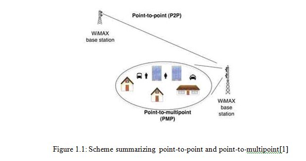
WiMAX Network Architectures
The MAC layer supports two modes, mesh and PMP (Point to Multi point). The BS (Base Station) communicates with several SSs using PMP mode and share uplink and down link channel information. All the SSs need to have a clear LOS to the BS in PMP mode. In mesh mode BS consist of net, Relay Stations (RSs), Subscriber Station and Mobile Station (MS). The mesh mode support of multi hop BS access the internet and RSs forward traffic to other RSs.
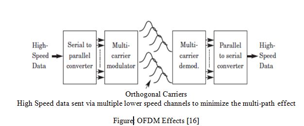
 OFDM Basics
OFDM belongs to multi carrier modulation technique that provides high data rates. In high data rate systems, delay spread is greater than symbol length. In NLOS systems, the delay spread will also be large and the wireless broadband system will suffer Inter Symbol Interference (ISI). To overcome this problem the multi carrier modulation divides the transmitted bit stream into lower stream. The individual sub streams are sent over parallel sub channels. The data rate of a sub channel is less than total data rate, so the sub channel bandwidth is less than total system bandwidth. Thus the ISI of each sub channel is small.
OFDM Features
The narrow band signals are less sensitive as compared to ISI and frequency selective fading.
In OFDM, Fast Fourier Transform (FFT) and Inverse Fast Fourier Transform (IFFT) operations ensure that sub channel do not interfere with each other.
OFDM provides robustness against burst error.
OFDM support less complex equalization as compared to the equalization in single carrier systems. Effective robustness can gain by multi path environments.
Mobility
Mobility support is available in IEEE 802.16e WiMAX standard. In BWA four scenarios support mobility.
Nomadic
In this scenario user is allowed to take a fixed subscriber station and reconnect from a different point of attachment.
Portable
The nomadic access scenario supports the portable devices such as PC card.
Simple mobility
In this scenario, the subscriber move at speed up to 60 kmph and interruptions are less than 1 sec during handoff.
Full mobility
The subscriber move at speed up to 120 Kmph and packet loss is less than 1 percent. It support seamless handoff and latency is less than 50 ms.
QoS in WIMAX
The QoS is a measure of how successfully the signals are transmitted from BS. The four parameters, as follows, are used to describe the QoS.
Bandwidth
The PHY Layer is a pipe between BS and the client terminal in WIMAX. The active clients are in parallel and share the overall system bandwidth.
Latency
Latency is the end to end packet transmission time, and occurs in physical layer chain. In IEEE 802.16 systems the latency is almost 5 ms. Latency is affected by how packets quid, different QoS protocols and user characterization are implemented.
Jitter
Jitter is the variation of latency over different packets and can be limited by number of packet buffering. Mobile terminal has little jitter control in wireless networks and it falls on the base station to ensure that different packets are received at different priority.
Reliability
Reliability leads to more complications in wireless networks as compared to fixed line ones. The problem arises specifically in mobile networks, where the radio wave propagates in mobile terminal with small antenna and low power in urban area
WiMAX Features for Performance Enhancement
WIMAX supports advanced features to improve the performance. These advanced feature support for multiple antenna techniques, hybrid-ARQ, and enhanced frequency reuse and multiple antenna technique.
Advanced Antenna Systems
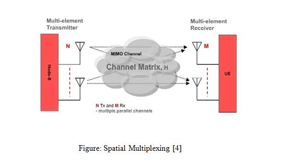
The WIMAX standard supports the multi antenna solution to improve system performance. The advanced antenna systems support the variety of multi antenna solutions, such as transmit diversity, Beam forming, and spatial multiplexing, all are used in WIMAX.
Diversity Schemes
The diversity scheme is a technique which is used for improving the reliability of a message signal. In this technique two or more communication channels are used with different characteristics. Diversity plays an important role in combating fading and co-channel interference.
In telecommunications, a diversity scheme refers to a method for improving the reliability of a message signal by using two or more communication channels with different characteristics. Diversity plays an important role in combating fading and co-channel interference and avoiding error bursts. It is based on the fact that individual channels experience different levels of fading and interference. Multiple versions of the same signal may be transmitted and/or received and combined in the receiver.
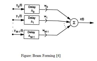
Beam Forming
Beam forming is a signal processing technique used in sensor arrays for directional signal transmission or reception. This is achieved by combining elements in the array in such a way that signals at particular angle experience constructive interference and while others experience destructive interference .Beam forming can be used at both the transmit and receive side to achieve spatial selectivity .The improvement compared with an OmnHYPERLINK “http://en.wikipedia.org/wiki/Omnidirectional”i HYPERLINK “http://en.wikipedia.org/wiki/Omnidirectional”directional reception/transmission is known as the receive/transmit gain (or loss).Beam forming can be used for both radio or sound waves. It has found numerous applications in radar, sonar, seismology, wireless communications, radio astronomy, speech, acoustics, and biomedicine. Adaptive beam forming is used to detect and estimate the signal-of-interest at the output of a sensor array by means of data-adaptive spatial filtering and interference rejection.
In this technique the antenna element focuses the transmitted beam in the direction of receiver, to improve the received Signal to Interference Noise Ratio (SINR). Beam forming supports; more coverage area, capacity, reliability, and support for both uplink and downlink.
 Spatial multiplexing
In spatial multiplexing the multiple independent streams are transmitted across multiple antennas. The spatial multiplexing is used to increase the data rate or capacity of the system. WiMAX also supports spatial multiplexing in uplink. The coding across multiple users in the uplink, supporting the spatial multiplexing, is called multi user collaborative spatial multiplexing.
 Modulation techniques
There are three main classes of modulation schemes, which are used to transmit the data.
Amplitude Shift Keying (ASK)
Frequency Shift Keying (FSK)
Phase Shift Keying (PSK)
All techniques are used in digital communication to convey the data. In phase shift keying the phase is changed to represent the data signal. There are two fundamental ways, which are used in phase shift keying.
Binary Phase Shift Keying (BPSK)
BPSK is sometimes called Phase Reversal Keying; it is the simplest form of phase shift keying. BPSK uses two phases, which are separated by 180 degree and known as two phase shift keying. This modulation is most robust from all PSKs modulation schemes due to its low probability of error. However, it gives lower data rates as compared to other modulation schemes. So for getting higher data rates we use QPSK and 16 QAM.
S1(t) = √2.Eb /Tb*cos(2πfct+π) = -√2.Eb /Tb*cos(2πfct) for binary
S1(t) = √2.Eb /Tb*cos(2πfct) for binary
Where, fc is the frequency of carrier
So, the signal can be represented by single basis function
Ф(t) = √2 /Tb *cos(2πfct)
Where 1 is represented by √EbФ (t) and 0 is represented by -√EbФ (t)
Related Work
There were some related work such as BER for BPSK modulation with 1Tx,2Rx Alamouti STBC(Rayleigh Channel).There are three receive diversity schemes –Selection combining, Equal Gain Combining and Maximal Ratio Combining. All the three approaches used the antenna array at the receiver to improve the demodulation performance .There are few receiver structure for 2*2 MIMO channel like Zero Forcing (ZF) equalization, Minimum Mean Square Error (MMSE) equalization, Zero Forcing equalization with successive Interface Cancellation (ZF-SIC).ZIF-SIC with optimal ordering .But Minimum Mean Square Error (MMSE) equalization with optimally ordered Successive Interference Cancellation gave the best performance.
Objective of this Thesis
In MIMO where the information is spread across multiple antennas at the transmitter and also receiver .We are discussing a popular transmit diversity scheme called Alamouti Space Time Block Coding (STBC). We are assuming the channel is a flat fading Rayleigh multi path channel and the modulation is BPSK. The Capacity of a MIMO channel with nt transmit antenna and nr receive antenna is analyzed. Capacity of MIMO the result dependences Capacity (bit/s/Hz), and the SNR (dB), in this simulation we are using the initial SNR = 2, results of simulation for capacity of MIMO 2×2, 3×3, 4×4 systems. The receiver structure of MIMO called Maximum Likelihood (ML) decoding which gives us an even better performance. We will assume that the channel is a flat fading Rayleigh multi path channel and the modulation is BPSK.
Introduction to this thesis paper
describes the Multiple Antenna Techniques such as the Diversity Scheme, Smart Antenna. An overview discussion on Multiple Input and Multiple Output (MIMO) system is also included.
explains about Alamouti Space Time Block Code which is stand for MIMO spatial multiplexing. The Rayleigh Fading Channel because are assuming that the channel is a flat fading Rayleigh multi-path channel And Alamouti STBC with two receive antenna.
illustrates the capacity of MIMO Vs. Signal to Noise Ratio (SNR) (db).
contains the Limitation of work, discussion and suggestion for future work.
Multiple Antenna Techniques
Introduction
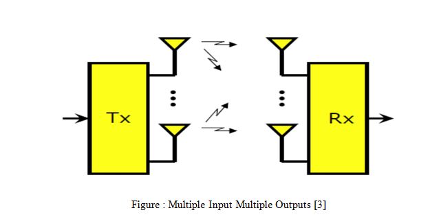
The Multiple Input Multiple Output (MIMO) technique uses an array of antennas for both transmitting and receiving end. Using MIMO techniques we can obtain better wireless communication as compared to other techniques. The electromagnetic waves transmitted from the antennas bounce around the environment, the receiver receives these electromagnetic waves from multiple directions, with varying delays. The delay varies since the different paths have different length. The Line of Sight (LOS) between the Base Station (BS) and the Subscriber Station (SS) is often very difficult to achieve, because the SS may be located indoors.
Multiple antenna techniques
Multiple antenna techniques are divided into three subclasses.
1. Diversity Schemes
2. Smart Antenna Systems (SAS)
3. MIMO Systems
Diversity Scheme
Diversity Scheme is a technique, which is used to improve the signal strength. In diversity scheme, two or more communication channels are used. Diversity plays an important role in reduction of fading and elimination of error burst. In diversity schemes multiple versions of the signal are transmitted and received. When these signals are transmitted the Forward Error Correction (FEC) code is added to different parts of the message. Different classes of diversity are given below.
Time Diversity
Multiple versions of the same signals are transmitted at different time instants. The FEC Code is added to the message. Then this message is spread in time before the transmission. In other words the elements of a radio signal transmitted at the same moment in time and these elements arrive at the receiver at different moments in time, because these signals uses different physical paths, through the use of receiving antenna technology known as rake receivers and multiple input multiple output (MIMO).
Frequency diversity
In this, the signal is transmitted using different frequency channels, such as spread spectrum. OFDM modulation is also used with sub carrier and FEC.
Space diversity
In Space diversity the signal is sent over different propagation paths. In wireless communication transmit diversity is used to transmit the signal and reception diversity is used to receive the signal. In this technique, if the antennas are much more than one wavelength away from each other, this is called macro diversity and if the antennas are in the order of one wavelength, then it is called micro diversity
Polarization diversity
In this technique multiple versions of signal are transmitted and received. It is used to minimize the effects of selective fading of the horizontal and vertical components of a radio signal. It is usually accomplished through the use of separate vertically and horizontally polarized receiving antennas.
Multi user diversity
Multi user diversity supports opportunistic user scheduling at either transmitter or receiver end. By using scheduling, the transmitter selects the best user from the candidate received according to the quality of each channel.
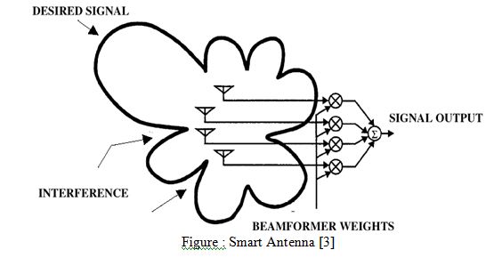
Smart Antenna System
The smart antenna system also called adaptive antenna system (AAS). In smart antenna system, by using signal processing techniques channel model attains channel knowledge to steer the beam towards the desired subscriber while transmitting null steering towards the interferer. The null steering cancels undesired portion of the signal and reduces the gain of radiation pattern obtained from adaptive array antenna. This is achieved by using Beam forming and null steering towards desired user. The process of combining the radiated signal and focusing it in the desired direction is called Beam forming.
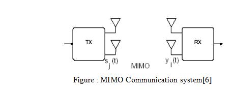
Multiple Input Multiple Output (MIMO) system
In MIMO technique BS and SS both have minimum of two transmitter and receiver, per channel as shown in figure 2.2.
Generally in 802.16, for diversity schemes, following three techniques are considered [3].
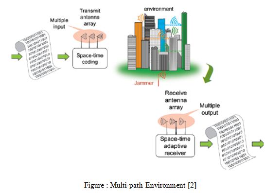
1. Space time coding
2. Antenna Switching
3. Maximum ratio combining
Space time coding technique
The 802.16 standard supports the Alamouti Scheme. In Space Time Coding, the information is sent on two transmit antennas. The information is sent consecutively in time and is called transmit information in time and space. A space–time code (STC) is a method employed to improve the reliability of data transmission in wirelessHYPERLINK “http://en.wikipedia.org/wiki/Wireless” HYPERLINK “http://en.wikipedia.org/wiki/Wireless”communication systems using multiple transmit antennas. STCs rely on transmitting multiple, redundant copies of a data stream to the receiver in the hope that at least some of them may survive the physical path between transmission and reception in a good enough state to allow reliable decoding.
Space time codes may be split into two main types:
Space–time trellis codes (STTCs) distribute a trellis code over multiple antennas and multiple time-slots and provide both coding gain and diversity gain.
Space–time block codes (STBCs) act on a block of data at once (similarly to block codes) and provide only diversity gain, but are much less complex in implementation terms than STTCs.
STC may be further subdivided according to whether the receiver knows the channel impairments. In coherent STC, the receiver knows the channel impairments through training or some other form of estimation. These codes have been studied more widely because they are less complex than their non-coherent counterparts. In no coherent STC the receiver does not know the channel impairments but knows the statistics of the channel. In differential space–time codes neither the channel nor the statistics of the channel are available.
Antenna Switching
Technique is used for capturing diversity gains. The purpose of the antenna switching is not to combine signals from the multiple antennas available, it is used to simply select the single antenna with the best channel gain at any given time. This is applicable to both downlink and uplink transmission.
Maximum Ratio Combining (MRC)
Maximum Ratio Combining (MRC) is the technique of diversity scheme which estimates channel characteristics for multiple antennas. MRC obtain diversity and array gain but does not involve spatial multiplexing in any way. In maximum ratio combining, the signal of each channel are added together and the gain of these channel is proportional to the Root Mean Square (rms) signal level and inversely proportional to the mean square noise level of these channels. Each channel has different proportionality constants, also known as ratio squared combining. [7]
Summary
To improve the performance in the Telecommunication field its very essential techniques .Now days without multiple antenna techniques it is impossible to think communication of data transfer .The Multiple Input Multiple Output (MIMO) technique uses an array of antennas for both transmitting and receiving end .Smart Antenna Diversity Scheme, MIMO are the techniques of multiple antenna. MIMO is the best from another two. In Space Time Coding, the information is sent on two transmit antennas. In maximum ratio combining, the signal of each channel are added together and the gain of these channel is proportional to the Root Mean Square signal level and inversely proportional to the mean square noise level of these channels.
ALAMOUTI Space Time Block Code for MIMO System
Introduction
In order that MIMO spatial multiplexing can be utilized, it is necessary to add coding to the different channels so that the receiver can detect the correct data.
There are various forms of terminology used including Space-Time Block Code – STBC, MIMO preceding MIMO coding, and Alamouti codes. Space-time block codes are used for MIMO systems to enable the transmission of multiple copies of a data stream across a number of antennas and to exploit the various received versions of the data to improve the reliability of data-transfer. Space-time coding combines all the copies of the received signal in an optimal way to extract as much information from each of them as possible. Space time block coding uses both spatial and temporal diversity and in this way enables significant gains to be made. Space-time coding involves the transmission of multiple copies of the data. This helps to compensate for the channel problems such as fading and thermal noise. Although there is redundancy in the data some copies may arrive less corrupted at the receiver.
When using space-time block coding, the data stream is encoded in blocks prior to transmission. These data blocks are then distributed among the multiple antennas (which are spaced apart to decor relate the transmission paths) and the data is also spaced across time.
A space time block code is usually represented by a matrix. Each row represents a time slot and each column represents one antenna’s transmissions over time.
Within this matrix, Sij is the modulated symbol to be transmitted in time slot i from antenna j. There are to be T time slots and nT transmit antennas as well as nR receive antennas. This block is usually considered to be of ‘length’ T.
MIMO Alamouti coding
A particularly elegant scheme for MIMO coding was developed by Alamouti. The associated codes are often called MIMO Alamouti codes or just Alamouti codes. The MIMO Alamouti scheme is an ingenious transmit diversity scheme for two transmit antennas that does not require transmit channel knowledge. The MIMO Alamouti code is a simple space time block code that he developed in 1998.The Alamouti code is a so called Space-Time Block Code (STBC). A block code is a code that operates on a “block” of data at a time and the output only depends on the current input bits. There are other codes, such as “convolution codes” whose output is dependent on the current input, and also on the previous inputs. These codes may not necessarily produce the same output for a given input, depending on what the previous input bits were. The main reason for using a block code is that typically it requires much less processing power to decode a block code than a convolution code.
ALAMOUTI Space Time Block Code
In Space Time Block code output only depends on the current input bits. In convolution codes, the output only depends on the current input bits and on previous inputs. The convolution code may not produce the same output for a given input, because previous input is involved. The block code requires less power, to decode a block code, as compared to convolution code.
The Alamouti coding is described by the following matrix and Y is the encoder output, while X 1 and X2 are the input symbols. The “*” denotes the complex conjugate.
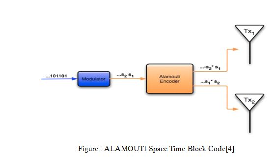
The figure is a block diagram of the transmitter module in MIMO system and using
the Alamouti code. The binary bits enter a modulator and are converted to “symbols”. A symbol from modulator is represented by complex numbers. This symbol can be transmitted directly in a single antenna, Single Input Single Output (SISO), system. In MIMO system the complex symbols are fed into the Alamouti encoder. The Alamouti encoder maps the symbols onto the transmitter by using the above given matrix. In this matrix, rows represent the transmit antennas, and columns represent the time. The element of the matrix tells what symbol is to be transmitted from a particular antenna. The Alamouti code works with pairs of symbols at a time. It takes two time periods to transmit the two symbols.
Rayleigh Fading Channel
The Rayleigh fading model is particularly useful in scenarios where the signal may be considered to be scattered between the transmitter and receiver. In this form of scenario there is no single signal path that dominates and a statistical approach is required to the analysis of the overall nature of the radio communications channel.
Rayleigh fading is a model that can be used to describe the form of fading that occurs when multi path propagation exists. In any terrestrial environment a radio signal will travel via a number of different paths from the transmitter to the receiver. The most obvious path is the direct, or line of sight path.
However there will be very many objects around the direct path. These objects may serve to reflect, refract, etc the signal. As a result of this, there are many other paths by which the signal may reach the receiver.
When the signals reach the receiver, the overall signal is a combination of all the signals that have reached the receiver via the multitude of different paths that are available. These signals will all sum together, the phase of the signal being important. Dependent upon the way in which these signals sum together, the signal will vary in strength. If they were all in phase with each other, they would all add together. However this is not normally the case, as some will be in phase and others out of phase, depending upon the various path lengths, and therefore some will tend to add to the overall signal, whereas others will subtract.
Rayleigh fading model has support for troposphere and ionosphere signal propagation. It is most applicable when there is no distinct dominant path along LOS, between the transmitter and receiver. In this regard, Jakes introduced a model for Rayleigh fading based on summing sinusoids. Jakes model works equally, if the single path channel is being modeled or multi path frequency-selective channel is required. The Jakes model also popularized the Doppler spectrum associated with Rayleigh fading and as the result this Doppler spectrum is often termed as Jakes spectrum.
Rayleigh fading is a reasonable model when there are many objects in the environment that scatter the radio signal before it arrives at the receiver. The central limit theorem holds that, if there is sufficiently much scatter, the channel impulse response will be well-modeled as a Gaussian process irrespective of the distribution of the individual components. If there is no dominant component to the scatter, then such a process will have zero mean and phase evenly distributed between 0 and 2π radians. The envelope of the channel response will therefore be Rayleigh distributed. Calling this random variable R, it will have a probability density function:
Where Ω = E(R2).
Often, the gain and phase elements of a channel’s distortion are conveniently represented as a complex number. In this case, Rayleigh fading is exhibited by the assumption that the real and imaginary parts of the response are modeled by independent and identically HYPERLINK “http://en.wikipedia.org/wiki/Independent_identically-distributed_random_variables”distributed zero-mean Gaussian processes so that the amplitude of the response is the sum of two such processes.
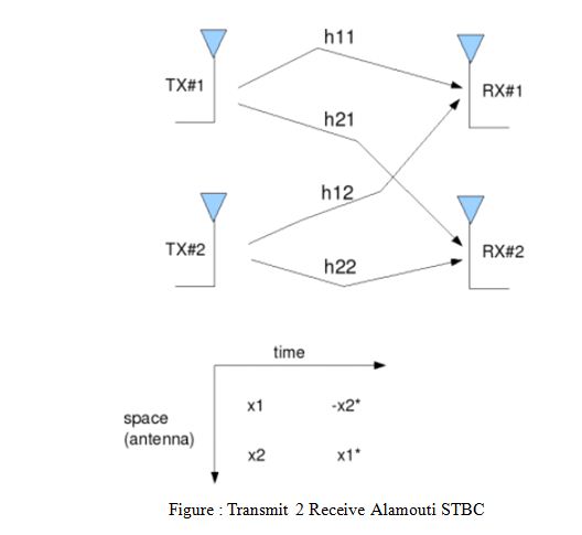
Alamouti STBC with two receive antenna
The principle of space time block coding with 2 transmit antenna and one receive antenna is explained in the post on Alamouti STBC. With two receive antenna’s the system can be modeled as shown in the figure below.
 The received signal in the first time slot is,
Assuming that the channel remains constant for the second time slot, the received signal is in the second time slot is,
Where
are the received information at time slot 1 on receive antenna 1, 2 respectively,
are the received information at time slot 2 on receive antenna 1, 2 respectively,
hij is the channel from ith receive antenna to jth transmit antenna,
x1, x2 are the transmitted symbols,
are the noise at time slot 1 on receive antenna 1, 2 respectively and
are the noise at time slot 2 on receive antenna 1, 2 respectively.
Combining the equations at time slot 1 and 2,
Let, define H=
To solve for, need to find the inverse of H.
The term,
Simulation Model
Generating random binary sequence of +1’s and -1’s.Group them into pair of two symbols. Code it per the Alamouti Space Time code. Multiply the symbols with the channel and then add white Gaussian noise. Equalize the received symbols Perform hard decision decoding and count the bit errors Repeat for multiple values of Eb/No and plot the simulation and theoretical results.
 Observation
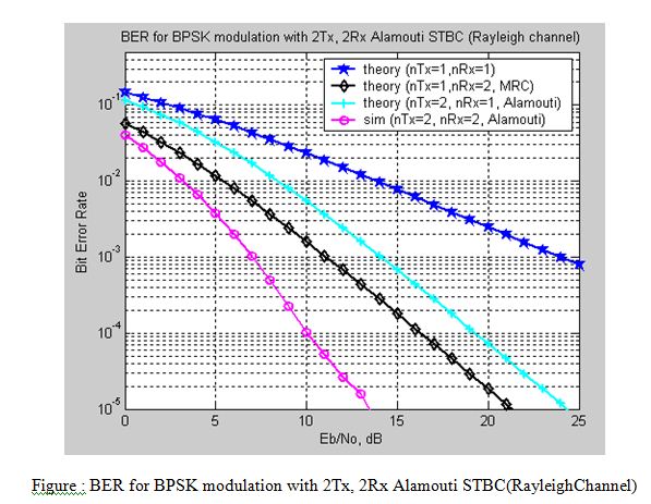
In Alamouti Space Time Block Coding with 2 transmitters and 1 receiver has around 3dB poorer performance. In Figure 3.3 the theoretical Alamouti calculation SNR is 24 db (approx.) and in the simulation SNR decreases 11 db (approx.). BER plot for nTx=1, nRx=2 Maximal ratio combining, the Alamouti Space Time Block Coding has around 5dB better performance.
Summary
BER performance is much better than 1 transmits 2 receive MRC case.In 1 transmitter and 2 receivers .The effective channel concatenating the information from 2 receive antennas over two symbols results in a diversity order of 4.In general, with m receive antennas, the diversity order for 2m transmit antenna Alamouti STBC.
ALAMOUTI Space Time Block Code for MIMO System
Introduction
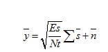
An overview of the channel capacities under different scenarios .Single input single output wireless channel capacity is considered first. Multiple channel capacity studies are inspected. MIMO capacity for different conditions is considered. Multi-Input Multi-Output communication system consisting of the following identities. s input symbols to be transmitted, Nt the number of transmit antennas, Nr the number of receiver antennas y the received symbol vector, H Nr x Nt MIMO channel matrix n noise with covariance matrix, E{nH}=N0INr
Capacity in AWGN
Capacity studies in communication started with Claude Shannon pioneered theorems. He defined capacity as the maximum mutual information between inputs and outputs of a communication channel. He then defined his coding theorem, which states that a code does exist that could achieve a data rate close to the capacity with a negligible probability of error. Shannon studies were related to the AWGN channel, wire lined channels. These channels do not fade the signals. Considering the wireless transmission, it is expected that the maximum supportable capacity is smaller than that of the wire lined channels. This is due to the multi-path and fading effects of the wireless communication channels. Capacity studies initially are done for flat fading channels.
The capacity of AWGN channel given the Bandwidth B and SNR g is given by the well known formula.
C=Blog2 (1+ g)
Shannon capacity can be considered as an upper limit for real systems. In wireless communication channel-fading information is important to be known at the transmitter or receiver side for better communication.
Capacity of Multi-channel Communications
Consider a Multi-Input Multi-Output communication system consisting of the following identities.
s input signal to be transmitted,
Nt the number of transmit antennas,
Nr the number of receiver antennas
y the received signal vector,
H is the channel response in the Nr x Nt MIMO channel matrix
n noise with covariance matrix, E{nnH}=N0INr
The relation between input and output is given by
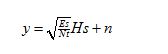 Es is the average transmits signal energy. If we choose Ts=1 then Es turns out to be the transmit power.
Deterministic MIMO channel capacity
Telstra has taken the role of Shannon for MIMO channel capacity studies; he defined the deterministic MIMO channel capacity as stated below
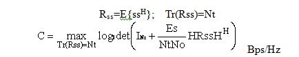
Channel knowledge available only at receiver
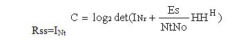
The channel capacity in the absence of the channel knowledge at the transmitter is given by the following formula.
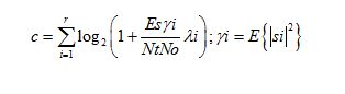
 Inserting HHH=QDQH in the above equation, an equivalent and simple expression is obtained as in (13)
C = ∑ Log2(1+ES /NtNo*λi)
i=1
r is the rank of the channel and lis are the positive eigenvalues of the HHH
In the case of an normalized orthogonal channel satisfying Nr=Nt=N, the capacity of the MIMO channel is given as
C = N log2 (1+ (Es/No))
That is the capacity of MIMO channel is equal to N times that of the SISO channel.
Channel knowledge available at the transmitter side case:
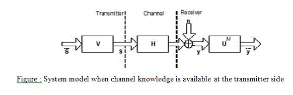 SVD of H yields H= UVH, inserting this into (11) and rearranging the parameters we get,
 Or this equation can be written as,
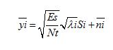
I=1..r, where r is the rank of HHH
The capacity of the MIMO channel is the sum of the SISO channels,
 Considering transmit power constraint the capacity formula reduces to,
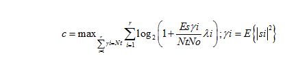 The capacity maximization problem can be solved using the lagrangian methods, hence leading to the results
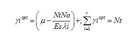
The optimal power allocation to the individual channels is found through an algorithm known as the Water pouring algorithm.
As can be seen from the formulas capacity of the MIMO channels increases when the channel knowledge is available at the transmitter, compared to the case in which receiver only has the channel information.
Capacity of the multiple input single output (MISO) and single input multiple output channels (SIMO).
Random MIMO channel capacity
Since the channel is random so the capacity is. In order to understand the capacity for the fading channels some definitions are needed. These are, ergodic capacity, outage capacity, outage probability,
Capacity is the expected value of the capacity over the distribution of the channel elements. It can be though as the mean information rate.
Outage probability: is the probability that given a transmission rate R and transmit power constraint the channel capacity cannot support a reliable communication
Pout = P(C£ R)
Outage Capacity:
Given an outage probability, the maximum information rate that can be supported by the communication channel is called the outage capacity of the channel.
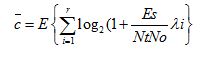
Capacity when the channel is known only to the receiver is given as:
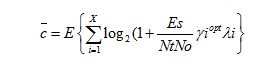
 The capacity when the channel is known to the transmitter is given as:
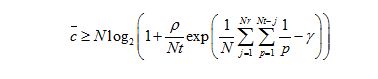
 A lower bound for the capacity is defined as [1],
 MIMO channel capacity in the presence of antenna correlation effect
When there is correlation between antennas at receiver or transmitter side, the channel matrix is expressed as,
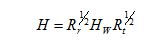 Where Rr and Rt are positive definite matrices showing the correlation effect between antenna elements. The elements of the R matrices can be found using
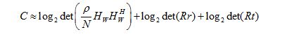
 At high SNR the capacity of the MIMO channel can be written as
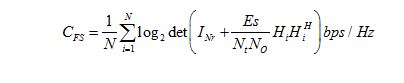
 Frequency selective MIMO channel capacity
If the channel is frequency selective, then the channel is divided into frequency flat sub-channels and the capacity of the each sub-channel is calculated using the frequency flat channel capacity formulas. The capacity of the frequency selective channel is the sum of each individual frequency flat channel. When the channel knowledge is available at the transmitter side, frequency flat channels uses the water pouring algorithm to distribute the power to the channel modes. In frequency selective channels, power must be distributed across space and frequency to make a more reliable communication. For deterministic frequency selective channels the capacity formula is given as in
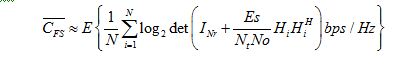
If the channel is random then the capacity for the frequency selective MIMO channel is defines as in .
Mutual Information and Shannon Capacity
Channel capacity was established by Claude Shannon in 1940s, by using the mathematical theory of communication. The capacity of a channel is denoted by C. The channel capacity C is the maximum rate at which reliable communication can be performed, without any constraints on transmitter and receiver complexity. Shannon showed that for any rate R < C, there exist rate R channel codes with arbitrarily small block error probabilities.
Thus, for any rate R < C and any desired non-zero probability of error ρe, there exists a rate R code that achieves ρe. The code may have a very long block length and encoding and decoding complexity may also be extremely large. The required block length may increase as the desired ρe is decreased or the rate R is increased towards C. Shannon showed that code operating at rates R > C cannot achieve an arbitrarily small error rate. So the error probability of a code operating at a rate above capacity is bounded away from zero. Therefore, the Shannon channel capacity is truly the fundamental limit to communication.
Capacity of MIMO system
MIMO system consists of multiple transmit and receive antennas interconnected with multiple transmission paths. MIMO increases the capacity of system by utilizing multiple antennas both at transmitter and receiver without increasing the bandwidth.
In the situation where the channel is known at both transmitters (Tx) and receiver (Rx) and is used to compute the optimum weight, the power gain in the kth sub channel is given by the kth value. i.e., the SNR for the kth sub channel equals
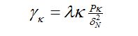
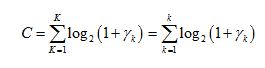
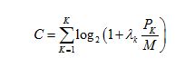
Where PK is the power assigned to the kth sub channel, λk is the kth value and σ2N is the noise power. For simplicity, it is assumed that σ2N = 1. According to Shannon, the maximum capacity of K parallel sub channels equals
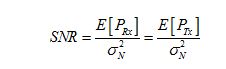
 Where M is the number of symbols and means SNR is defined as
Given the set of evalues { λk }, the power PK allocated to each sub channel k is determined to maximize the capacity by using Gallager’s waterfilling theorem such that Each sub channel is filled up to a common level D, i.e.
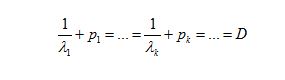 With a constraint on the total Tx power such that
 Where, PTX total transmitted power. This means that the sub cannel with the highest
Gain is allocated with the largest amount of power. In the case where 1/ λ, k >D then PK =0
When the uniform power allocation scheme is employed, the power PK is adjusted according to
P1 = ⋯ = PK
Thus, in the situation where the channel is unknown, the uniform distribution of the power is applicable over the antennas. So that the power should be equally distributed between the N elements of the array at the Tx, i.e.,
Pn= PTX/N; n=1…..N
Capacity Analysis using Shannon Capacity
MIMO system consists of multiple transmit and receive antennas interconnected with multiple transmission paths. MIMO increases the capacity of system by utilizing multiple antennas both at transmitter and receiver without increasing the bandwidth. In the situation where the channel is known at both transmitter (Tx) and receiver (Rx) and is used to compute the optimum weight, the power gain in the kth sub channel is given by the kth value, i.e., the SNR for the kth sub channel equals.
The capacity of MIMO system is given as follows
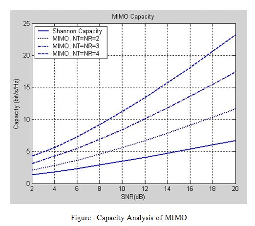
 By implementing the above equation using mat lab, following result is obtained
 Observation
Figure 4.3shows, an analysis of the capacity of the system having multiple transmitters and receivers. The capacity of a MIMO system has been plotted against SNR in dB. It is clear that with increase in the number of antennas at the both sides capacity increases linearly i.e. with nt=4 and nr=4, we have achieved highest capacity in MIMO systems.
Summary
MIMO system transmits two or more data streams in the same channel. The data streams are sent at the same time. MIMO System are also used to obtain the goal of evaluating the capacity of a system using N transmit and M receive antennas. Increasing number of antennas at either side of the MIMO system will have same effect in raising the capacity.
Discussion and Suggestion for future work
Discussion
Modern wireless systems requires high data rate. The MIMO techniques are physical layer based and essential part of the IEEE 802.16e-2005. The Simulation result with 2 transmit antenna and 2 receive antenna using Alamouti STBC code is better than Theoretical value with 2 transmit antenna and 1 receive antenna using Alamouti code.In MRC case with 1 transmitter and 2 receiver is much better than theoretical 1 transmit antenna and 1 receive antenna .This is because the effective channel concatenating the information from 2 receive antennas over two symbols results in a order of 4.with m receive antennas, the diversity order for 2 transmit antenna Alamouti STBC is 2m. Moreover the results of MIMO capacity shows that increase in number of antennas at the both side’s capacity increases linearly. Figure 4.3 shows that, when nt=4 and nr=4 it achieves the highest capacity as compared with nt=2 and nr=3 and nt=3 and nr=2 respectively in MIMO system. Increasing the number of antennas at either side of MIMO system will have the same effect of raising the capacity. Matlab 6.5 is used for Simulation.
Suggestion for future work
Multiple Antennas is indeed a very vast topic and myriad scopes are there to execute research. This book is rather an introductory concept about the multiple antennas and an overview and performance analysis of MIMO .There are three techniques for MIMO. This book is worked with Alamouti Space time block coding .BER performance for BPSK modulation with nTx, nRx Alamouti STBC can be improved. In future,This simulated bit error rate performance results can be tested and verified practically. Further research can be helpful to make it more efficient and reliable in performance.
Limitations
Wireless Cellular networks are usually interference-limited and different data streams on different antennas are equivalent to more users in system .If Ntx=Nrx, multiple antennas at receiver allow separation of all desired data streams. If Ntx<Nrx,multiple antennas at receiver additional don’t allow separation of all desired data streams. Capacity of MIMO with increasing transmitter and receiver can be tested using matlab simulations .Here 4 transmitter and receiver is used for simulation.