In the discrete-time situation, autocorrelation, also known as serial correlation, refers to the degree of correlation between the values of the same variables across multiple observations in the data. It assesses the relationship between the lagged version of a variable’s value and the original version in a time series. It’s the relationship between a signal and a delayed duplicate of that signal as a function of time. It’s the similarity of observations as a function of the time lag between them, to put it another way.
Autocorrelation is similar to correlation in that it utilizes the same time series twice: first in its original form and then lagged by one or more time periods. It’s frequently used in conjunction with the autoregressive-moving-average (ARMA) and autoregressive-integrated-moving-average models (ARIMA). Autocorrelation analysis is a mathematical method for detecting recurring patterns, such as the presence of a periodic signal masked by noise or the identification of a signal’s missing fundamental frequency suggested by its harmonic frequencies.
Autocorrelation analysis also aids in the discovery of repeating periodic patterns, which may be utilized as a technical analysis technique in the financial markets. It’s frequently used in signal processing to examine functions or sequences of values, such as time-domain signals. Autocorrelation is most commonly addressed in the context of time series data, which includes observations at several periods in time (e.g., air temperature measured on different days of the month).
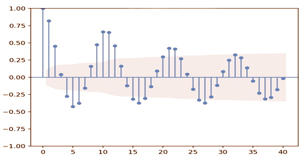
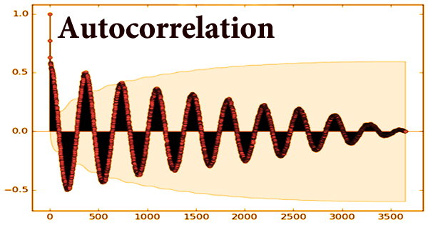
Autocorrelation is defined variously in different fields of study, and not all of these definitions are comparable. In certain domains, the terms autocovariance and autocorrelation are interchangeable. Autocorrelation may, of course, be a helpful tool for traders, particularly technical analysts. The autocorrelation value varies from -1 to 1. Negative autocorrelation is defined as a number between -1 and 0. Positive autocorrelation is defined as a number between 0 and 1. Autocorrelation can be beneficial in technical analysis for the equity market since it provides information about the trend of a collection of historical data.
Because it assesses the link between a variable’s current value and its previous values, autocorrelation is also known as lagged correlation or serial correlation. When the observations are linked in some other manner, it can also happen with cross-sectional data. When observations are reliant on factors other than time, autocorrelation can develop. It can pose issues in traditional studies that presume observation independence (such as basic least squares regression).
Autocorrelation analysis looks for a pattern or trend in a time series by measuring the connection between data at different periods in time. If the model is improperly defined, autocorrelation of the regression residuals might arise in a regression study. The Pearson correlation between values of the process at various times, as a function of the two times or the time lag, is the autocorrelation of a real or complex random process in statistics.
A complete positive correlation is represented by an autocorrelation of +1. An autocorrelation of -1, on the other hand, denotes a complete negative correlation. Autocorrelation can be positive or negative, much like correlation. Positive autocorrelation indicates that when a time interval increases, the delayed time interval increases proportionately. There can be a nonlinear link between a time series and a lagged version of itself even if the autocorrelation is negligible.
Normalizing the autocovariance function to get a time-dependent Pearson correlation coefficient is standard practice in several areas (e.g. statistics and time series analysis). Because technical analysis is primarily concerned with the patterns of, and correlations between, asset prices using charting techniques, autocorrelation can be beneficial. Normalization is generally abandoned in other areas (e.g., engineering), and the words “autocorrelation” and “autocovariance” are used interchangeably.
Autocorrelation may be used by technical analysts to determine how much previous prices for an asset have on its future price. Negative autocorrelation, on the other hand, means that a rise in one-time intervals causes a proportional reduction in the delayed time interval. Autocorrelation can be used to identify whether or not a stock has a momentum factor. If a stock with a high positive autocorrelation has two days of significant increases in a row, it’s realistic to predict the stock to continue to rise for the next two days.
The normalization is essential because the interpretation of the autocorrelation as a correlation gives a scale-free measure of the intensity of statistical dependence, and it affects the statistical characteristics of the calculated autocorrelations. When evaluating a set of historical data, it is important to test for autocorrelation. In the stock market, for example, stock prices on one day might be strongly linked with stock prices on another day. It, on the other hand, gives minimal information for statistical data analysis and does not reveal the stock’s real performance.
Information Sources: