Atomic Absorption spectroscopy is one of the excellent analytical instruments for the analysis of the chemical composition of samples. Walsh was first introducing the instrument as a general purpose, now it is very popular analytical technique to determination of different elements. It is based on the absorption of UV or visible light by gaseous atoms and suitable for the analysis of metals. A very large number of elements can be analyzed for at trace levels and AAS has a very wide range of applications. More than seventy elements can be determined in almost any matrix such as heavy metals in body fluid, polluted water, foodstuffs, soft drinks, analysis of metallurgical and geochemical samples and the determination of many metals in soils. Detection limits in the range of ppb to ppm level.
Atomic absorption spectroscopy (AAS) is the appropriate term used when electro-magnetic radiation (EMR) is absorbed or emitted by atoms and measured. All atoms can absorb EMR and the wavelengths at which EMR is absorbed or emitted is exclusive for a particular chemical element. AAS is a quantitative method of analysis that is used to analyze many metals and a few non-metals.
Theory
Atomic absorption (AA) spectroscopy uses the absorption of light to measure the concentration of gas phase atoms. Since samples are usually liquids or solids, the analytic atoms or ions must be vaporized in a flame or graphite furnace. The amount of absorption in their elemental form, elements will absorb UV or visible light when they are excited by heat and make transitions to higher electronic energy levels. The AAS instruments looks for a particular element by focusing a beam of UV light at specific wavelength through a flame and into a detector. The sample of interest is aspirated into the flame. If that metal present in the sample, it will absorb some of the light, thus reducing its intensity. The instrument measures the change in intensity. Concentration measurements are usually determined from a working curve after calibrating the instrument with standards of known concentration.
In normal condition, atom exists in the ground state. Although we can not measure the precise energy state for an atom, we can measure changes its energy relative to its ground state. Certain processes can change the energy state for an atom. This change in energy is ∆E, this is the energy absorption by an atom. From the quantum mechanics we found,
∆E = h/λ
Where h is planks constant, λ is the specific wave length absorbed by an atom. For an example, calcium absorbs light of a wavelength of 422.7 nm. Iron absorbs light at 248.3 nm.
The success or failure of analysis depends upon excitation and getting appropriate resonance line. The relationship between the ground-state and excited-state populations is given by the Boltzmann equation:
N/ N = (g/g) e
Where,
N1 = Number of atoms in the excited state
N0 = Number of atoms in the ground state
g/g = Ratio of statistical weights for ground and excited states
k = Boltzmann constant (1.38×10⁻²³JK-1)
ΔE = Difference between energy level = Eupper – Elower
T = Temperature in Kelvin scale
It can be seen from this equation that the ratio N/N is dependent upon both the excitation energy ΔE and the temperature T. An increase in temperature and a decrease in ΔE (i.e. when dealing with transitions which occur at longer wavelengths) will both result in a higher value for the ratio N/N. An increase in temperature increases the efficiency of atomization. The total amount of energy absorbed by the sample element to achieve the excited state is equivalent to the number of electrons available-in other words, to the concentration of the element in the sample. This forms the basis of the Atomic Absorption Spectroscopy, viz. the measurement of the amount of energy of the correct wavelength necessary to elevate the metal atoms from ground state to the excited state
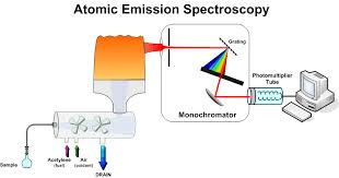
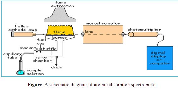
Simple diagram of AAS
The atomic absorption spectrometer consists of a source of light, an atom cell, a monochromator and a read-out system. An atomic absorption spectrophotometer generates a source of light to be absorbed and passed through the gaseous state of the sample that has been sprayed into a flame and the analytes are determined by measuring the absorption of the constant intensity of EMR that passes through the flame.
Light source
In most atomic absorption methods, the most widely used light source is the hollow cathode lamp because that source of light can provide a narrow line source. A hollow cathode lamp is made of a glass tube with a cathode inside made of the element being analyzed and a suitable anode. The closed glass tube contains an inert gas, typically neon or argon at a pressure of 1-5 torr. When a high voltage of about 600 V and 2-30 mA is applied between the electrodes the inert gas becomes ionized and the positive ions are accelerated toward the cathode. They strike the cathode with enough energy to “sputter” metal atoms from the cathode into the gas phase. Manny of the sputtered atoms are in excited states, they emit photons of few spectral lines characteristics of that element (for instance, Cu 324.7nm and a couple of other lines; Se 196 nm and other lines etc.) This atomic radiation is of exactly the same frequency as that absorbed by atoms of the analyte in the flame or furnace. The light is emitted directionally through the lamp’s window, a window made of glass transparent in the UV and visible wavelengths.
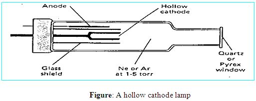
More advantages to hollow cathode lamps is that they are simple to operate, they produce a stable and intense light, they are economical and that hollow cathode lamps can be made for all chemical elements that can be analyzed by atomic absorption.
Atom cell
The most widely used atom cell is the flame. The flame is characterized by the gases involved, the temperature of the flame itself, the flow of gases, the form in which the gases are mixed, its shape and size. Air-acetylene (operating temperature of 2300o C) and nitrous oxide-acetylene (operating temperature of 3000o C) are the most commonly used flames.
Atoms are formed within the flame by the atomization process. The dissolved sample in solution is heated to the point of the solvent evaporating, followed by the solids being heated to high enough temperatures to decompose into compounds and eventually decompose into individual atoms. The atoms in the gaseous state then absorb EMR from the light source
Light disperser
The purpose of the light disperser or monochromator is to isolate a single atomic resonance line from the spectrum of lines emitted from the light source. The desired spectral line is chosen with the preferred wavelength and bandwidth by an appropriate monochromator’s setting named grating. A grating is a reflective surface, scored either mechanically or holographically with parallel grooves that can be designed for different wavelength regions. Generally, most of the instruments are equipped with two gratings with the goal to cover a wavelength range from 189 to 851 nm, which is used in atomic absorption.
Detector and read out system
The most common type of detector is the photomultiplier tube. The photomultiplier produces an electrical signal which is proportional to the intensity of EMR of the wavelength separated by the light dispersing monochromator.
The signal from the detector is transferred to the computer and the analytical result (output) is seen on the monitor of the computer. There is a fundamental problem with readout systems. Dark current (current flowing in the absence of light) within the photomultiplier and dc current caused by light that is not from the hollow cathode tube. These interferences pose an analytical problem because they are not differentiated from the signals that are given off from the light that comes for the analyte. This problem is avoided by “coding” the signals of light from the hollow cathode tube. Because the invalid signals (dark current and interfering light) are not “coded”, they are rejected from the readout system
Sensitivity and limit detection
There are certain factors that decrease the sensitivity such as excessive noise in the source, having a large number of reflecting surfaces and turbulence in the optical path. Some ways of minimizing noise is by providing a stable flame and using a low noise detection system. AAS is a very sensitive analytical method that can detect as low as 10-12 grams
Atomic spectroscopy interferences
There are two common types of interference that reduce the concentration of free gas-phase atoms, ionization and the formation of molecular species or refractory compounds.
Ionization interference
Higher temperature environment can lead to ionization of the sample atoms; the concentration of atoms in a flame is reduced if ionization occurs.
M (g) → M+ (g) + e
As a result ionization leads to reduced signal intensity, as energy levels of ions are different from those of the parent ions.
Preventing ionization
Ionization of the analyte element can be suppressed by adding an element that is more easily ionized. Ionization of the added element results in a high concentration of electrons in the flame. So enhance the absorption by gaseous atom. In analysis of alkali and alkaline earth metals this effect can be important and it is necessary to control variations in ionization equilibria with concentration by adding an excess of another easily ionized element, which is not involved in the analysis, e.g. Cesium and potassium are common ionization suppressor and that are added to analyte solutions.
Preventing refractory compounds formation
Elements that form stable compounds are not completely atomized at the temperature of the flame or graphite furnace. For an example calcium in the presence of phosphate forms stable Calcium Phosphate. This refractory molecule interfere the measurements of Calcium.
3 Ca2+ + 2 PO43- Ca 3(PO4)2
Formation of the refractory molecules can be prevented or reduced by adding releasing or chelating agents. For calcium measurements adding releasing or chelating agents for producing less stable compounds:
Addition of a releasing agent for the determination of calcium:
Ca3 (PO4)2 + 2 LaCl3 3 CaCl2 + 2 LaPO4
Addition of a chelating agent for the analysis of calcium:
Ca3 (PO4)2 + 3 EDTA 3 Ca (EDTA) + 2 PO43-
Interference in flame
Solvent effect
The processes actually occurring in the flame and which generate atoms in their ground states are rather a complex. The necessity to precisely control all conditions of analysis is illustrated by the fact that the fuel/oxidant flow rates affect the efficiency of aspiration and hence, the degree of atomization in the flame and that the combustibility of the solvent affects desolvation and subsequent atomization.
The solvent dependence of absorption is, in fact, one example of the occurrence of important matrix effects in AAS. In general, the efficiency of atom generation in a flame depends to some extent on the nature of every species in the analyte solution. It is therefore, desirable to prepare all solutions for analysis for a particular element in a medium of as constant a composition as possible. Where this is not possible, the method of standard addition must be used. This procedure involves addition of various known amounts of the element being determined to the unknown solution, construction of a standard curve and extrapolation of the curve to find the initial concentration.
Anion interference
Anions such as phosphate and sulphate form rather in volatile salts with many metals and consequently can inhibit vaporization in the flame. Such problem may overcome by the use of a hotter or more reducing (fuel rich) flame. Vaporization interference may also be overcome by addition of releasing agents, which either interact with the anion or form a complex of the cation, which is no longer affected by the anion. Phosphate interference may be diminished by addition of lanthanum salts in excess, as La3+ preferentially forms an in volatile phosphate, or by addition of EDTA to form e.g. [Ca EDTA] 2-, which is readily volatilized in the flame.
Ignition, flame conditions and shut down
The AAS flame ignition involves on first the fuel then the oxidant and then lighting the flame with the instrument’s auto ignition system. De-ionized water or a dilute acid solution can be aspirated between samples. An aqueous solution with the correct amount of acid and no sample is often used as the blank.
Careful control of the fuel/air mixture is important because each element’s response depends on that mixture in the burning flame. Optimization is accomplished by aspirating a solution containing the element and then adjusting the fuel/oxidant ratio, until the maximum light absorbance is achieved.
Shut down involves aspirating de-ionized water for a short period and then closing the fuel off first. Modern instruments control the ignition and shutdown procedures automatically.
Applications of AAS
AAS is considered to be one of the best quantitative methods of analysis for metals. AAS methods have been useful in the analysis of plant materials, biological materials, analysis of food and beverages, chemical products, and environmental studies
The uses of AAS have led to major discoveries in the field of astrophysics. A considerable amount of our knowledge about the cosmos comes from our empirical understanding of spectral lines emitted by objects in outer space. Studying the wave lengths of EMR emitted by astronomical objects gave insight to the chemical composition present in these celestial bodies and their respective velocities. Other information such as the densities, temperatures, abundances of elements can be acquired by studying the intensities of spectral lines that are emitted. The Doppler Effect (the change in the apparent frequency of a wave as observer and source move toward or away from each other) provides evidence that the universe is expanding because of red shifts emitted
UV- Visible spectrophotometry
The basis of the photometric method is that the color of a solution varies with the concentration of the metal complexes. The color of a solution is the indication of complex formation between the metals and the added reagent. The spectrophotometric method deals with the monochromatic light source. The chief advantage of the spectrophotometric method is that it provides a sample means for determining minute quantities of substances. This method is based on the theory of Lambert and Beer.
Theory
When a monochromatic light falls upon a medium a portion of incident light is absorbed and a portion of light is reflected. The logarithmic ratio of the absorbed light (lo) and transmitted light (I) is known as the absorbance of the solution and is represented by “A”. This can represent as
log lo/I = A ………… (I)
Lambert’s law states that “If a monochromatic radiation passes through a transparent medium, the absorbance of the solution is proportional to the thickness of the medium.”
If A is the absorbance of the solution, l is the thickness of the medium, so according the law,
A ά l —————— (II)
Beer’s law states that “When a monochromatic radiation passes through a transparent medium the absorbance of the solution is proportional to the concentration of the medium.” i.e.
If A is the absorbance of the solution, C is the concentration of the medium, so according the law,
A ά C ——————- (III)
The combination of the equation (II) & (III)
A ά C .l
A = ЄC .l (Є = Constant, it known as molar absorptivity). This law is known as Beer-Lambert law. Here, l is also constant for a cell. Therefore by measuring the absorbance of a solution, the concentration of the solution can be measured by the equation.
Validity of the law
For valid application of the law the following conditions should be fulfilled. 1. The sample solution should be diluted. 2. The used light should be monochromatic. 3. The applied radiation should be reflected or scattered before absorption. 4. Molecules or ion in solution should not remain associated, dissociated, hydrated or complex. 5. The solute should not remain in equilibrium with other solutes in solution and the pH value of the solution should not be changed in any way.
If the law is valid a plot between absorbance and concentration is a straight line passing though origin. But when the solution is concentrated beyond the desired level, the curve deviates from the straight line. This deviation may be positive or negative but in most cases the deviation becomes negative which is shown in figure.
Experimental
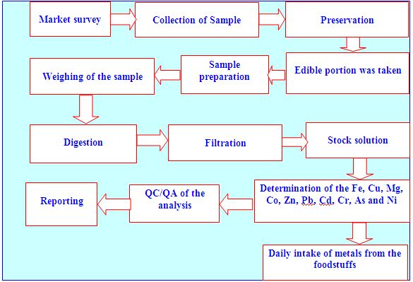
This research work was conducted through the inception and implementation of the following research plan which has been represented in the form of flow chart according to the sequence of the works.
Chemicals, reagents and glass wares
1000 ppm reference standard solution of Fe, Cu, Mg, Co, Zn, Pb, Cd, Cr, Ni, and As were collected from BDH, UK. CuSO4.5H2O, MgSO4.7H2O and [Fe (NH4)] (SO4)2.12 H2O of analytical grade (Merk) were used. Pure concentrated HNO3 and HClO4 were obtained from Merk. Redistilled water (RDH2O) was used throughout the experiment. Demonized water was used during preparation of any solution. Concentrated HCl and NH4OH, NH2OH.HCl, Orthophenanthroline, Buffer solution, Congo red paper, Na2EDTA, (NH4)2C2O4, Sodium dieheyldithiocarbamate (Copper reagent), CCl4, Cresol red, KI solution, NaBH4 solution etc. were collected as analar grade. All glassware were washed and rinsed with redistilled water, washed glassware were placed in 20% nitric acid for 48 hours and then rinsed extensively with distilled and redistilled water.
Precaution against contamination
For analysis of trace level of analyze, it is necessary to keep the blank values as low as possible [14]. Hence glassware should be cleaned and dried in such a manner to ensure that contamination from glassware does not occur. The cleanliness of the environment in which the analysis is performed, has a direct effect on the accuracy and precision of the method. In order to achieve accurate results, all glassware and digestion vessels was cleaned immediately prior to use with dilute HNO3 (20%) and then rinsed with RDH2O
Samples under analysis
The following sets of samples (one hundred and seventy items) available in Chittagong of Bangladesh have been analyzed.
Set A: Meats, organ meats, meat products and eggs (Chapter-3)
Set B: Pulses, spices and sauces (Chapter-4)
Set C: Fruits, jellies and juices (Chapter-5)
Set D: Hot drinks, chips and cereals (Chapter-6)
Set E: Tobacco cigarettes and other tobacco products (Chapter-7)
Set F: Edible oils and ghee (Chapter-8)
Sampling
The significance of an analysis depends to a large extent on the sampling program. An ideal sample should be one which is both valid and representative. To ensure these conditions sample collection was made through a process of random selection.
Sample preparation (Methodology)
The origin of samples of each group was different, in all cases the only consumable parts of the foods were taken for metal analysis. All the samples were pretreated to destroy organic matter, because the technique used for metal analysis i.e. atomic absorption spectrophotometer required clear organic matter free and transparent solution. Samples were washed (if necessary) with redistilled water (RD H2O), so that there was no dust particle seen on samples and samples were cleaned visually. The samples were dried at room temperature to a constant weight. The dried samples were then mixed well, which used for wet acid digestion. In order to complete digestion of such foodstuffs, several methods have been performed. Among them acid digestion method is widely used method to maximize spike recovery, precision and accuracy
Samples were performed to digest by 5:1 mixtures of HNO3 and HClO4 because this method gave the better percentage of recovery (83 – 103%) of the metals that have been studied in the study.
Analytical techniques
Concentration of essential and toxic metals in the studied food samples were measured by AA-240 Fast sequential atomic absorption spectrometer (VARIAN) and GTA-120 graphite tube atomizer, AA-240 Zeeman atomic absorption spectrophotometer. The instrumental conditions for analysis are given in Table 2.2. Air-acetylene flame and helium as carrier gas were used in AAS. The burner height and orientation was adjusted for maximum absorbance while aspirating a standard solution. This instrument that has been used can direct readout of concentration, integration, measurement of peak height. All the spectroscopic measurements of the standard metal solutions as well as the sample solutions were done at their respective wavelength of maximum absorptions, גmax
While the concentration of Fe, Cu, and Mg were determined in meat samples by UV-visible double beam spectrophotometer, model Cintra, Australia.
Standards
Certified atomic absorption reference standards of lead, cadmium, chromium, arsenic, nickel, iron, copper, magnesium, cobalt, zinc solution containing 1000 mg of respective metal ion per liter were obtained from BDH, UK. For the purpose of the calibration curve, the working standard solutions were prepared immediately before their use, by proper dilution of the certified standard solution with 2% HNO3.
Preparation of reagents
I. 10% NH2OH.HCl Solution: 10% NH2OH.HCl was prepared by dissolving 10g NH2OH.HCl in 100mL water.
II. Orthophenanthroline solution: Orthophenanthroline solution was prepared by dissolving 1.2g Orthophenanthroline powder in one litre volumetric flask and diluted up to the mark with distilled water. The powder was fully dissolved by shaking. The Orthophenanthroline solution was used throughout the present investigation.
III. NH4OH.H2O: 1:1 (14.3 N Ammonia solution and distilled water were used for the preparation of 1:1 NH4OH/ H2O solution)
IV. Buffer solution: Buffer solution (pH=5) was prepared by dissolving 27.3 g of NaOOCCH3.3H2O in water containing 60mL of 1NHCl and diluted with distilled water to 1litre.
V. Congo red paper: 10 mg Congo red paper was dissolved in 10mL ethanol. This is known as Congo red solution. Some pieces of filter paper were dipped into the Congo red solution and than dried. These prepared Congo red papers were used throughout the studies.
VI. Ferric ammonium sulfate solution: 0.864 g A.R. Ferric ammonium sulfate was dissolved in a 1litre volumetric flask with distilled water and 5mL concentrated HCl was added. The total volume was made 1000mL with distilled water. In this solution 1 mg contains 0.1 mg Fe3+. This solution was kept as stock solution and used for the preparation of calibration curve of iron.
VII. Versenate citrate mixture: Versenate citrate mixture was prepared by dissolving 20 g ammonium citrate and 5 g disodium salt of EDTA in a 100mL volumetric flask with distilled water. This solution was used throughout the studies.
VIII. 1% Sodium diethyldithiocarbamate solution: 1% Sodium diethyldithiocarbamate solution was prepared by dissolving 1 g sodium diethyldithiocarbamate in a 100mL volumetric flask with distilled water. This solution was used throughout the studies.
IX. Cresol red solution: Cresol red solution was prepared by dissolving 10 g cresol red powder in 10mL ethanol.
X. Standard copper sulfate (CuSO4.5H2O) solution: 0.3928 g copper sulfate was dissolved in a 1litre volumetric flask with distilled water and 5mL concentrated H2SO4 was added. The total volume was made 1000mL with distilled water. This solution was kept as stock solution. Solutions of different concentration were made from the stock solution by proper diluting for the preparation of copper calibration curve.
XI. Buffer solution: Buffer solution (pH=10) was prepared by dissolving 0.75 g of A. R. ammonium chloride in water containing 5mL concentrated ammonia solution and diluted to100mL with distilled water.
XII. Solo-chrome black solution: 0.1 percent solution was prepared by dissolving 0.1 g solo-chrome black in a 100mL volumetric flask with methanol. The solution was warmed and then it was filtered.
XIII. Standard magnesium sulfate solution (MgSO4.7H2O) solution: 0.1 g magnesium sulfate was dissolved in a 100mL volumetric flask with distilled water. 1mL concentrated HCl was added. The total volume was made 100mL with distilled water. This solution was kept as stock solution. Different concentration was made by diluting the stock solution for the preparation of magnesium calibration curve
Preparation of calibration curves
A calibration curve of the respective metal was prepared by plotting the absorbance against concentration of the standard solutions. Metal concentrations of the samples were measured with the help of these calibration curves covering the optimum linear absorbance range. In all absorbance measurements, the reading was taken after instrumental zero has been adjusted. By measuring the absorbance of the standard solution for respective metal, a calibration curve was automatically constructed and displayed in the monitor of spectrophotometer. The calibration curve was checked periodically by measuring absorbance and concentration of independent standard solutions according to the sensitivity of the instrument. When the measured value of the independent standard metal solution showed deviation more then ten percent from its known concentration then recalibration was done for the respective metal. Thus the accuracy and precession of the analytical data were strictly followed throughout the present study.
UV-visible spectrophotometric measurement
The necessary standard metal solutions were prepared in ppm level for constructing calibration curves of Mg, Fe and Cu by UV-Visible spectrophotometer (Table 2.1). After developing the color of the sample solution as well as the sample blank are taken in 1 cm cell, the absorbance and concentration data was measured by the instrument. Table: Standard compounds used for the λmax and Calibration Curves
Metal | Standard Compounds Reference Measured Slit Width λmax/nm λmax/nm /nm |
| Fe Cu Mg | FeNH4(SO4) 2 510 509.23 1.5 CuSO4.5H2O 435 435.62 1.5 MgSO4.7H2O 520 527.25 1.5 |
Calibration curve for Iron
Stock solution of Fe [2.2.9 (VI)] was used for calibration purpose. In this solution, 1mL contains 0.1 mg of Fe3+. From this solution different volume (0.1mL, 0.2mL, 0.3mL, 0.6mL, 1mL) were taken in different 100mL volumetric flask with 50mL RDH2O and 2mL conc for preparation of calibration standards. HCl was added in each of the flask. NH2OH.HCl (1 mL) was added into the solution of each flask. The congo red paper was turned into bluish. Conc. NH4OH solution was added drop wise until alkaline, now congo red paper became just red. 5mL Buffer (pH=5) solution was added in each of the flask. If necessary the solution was filtered through a whatman–filter paper and made the total volume 100 mL with RDH2O. An orange red color developed and its absorbance at 509.23 nm was measured within one hour of color development.
A blank solution was prepared by using all the reagents except ferric ammonium sulfate solution by similar procedure and was used to make the spectrophotometer reading zero before measuring the absorbance of every standard solution. The calibration curve was prepared by plotting the concentration of standard solution versus corresponding absorbance.
Standards
Concentration range = 0 – 1.6 ppm
Absorbance range = 0 – 0.720 Statistical data y= mx + c
Iron determination
5 mL stock solution was taken into a 100 mL volumetric flask. 10% NH2OH.HCl solution (1 mL) was added for the reduction of Fe3+ to Fe2+. Orthophenanthroline solution (5 mL) along with a piece of congo red paper added in the solution. The congo red paper was turned into bluish then NH4OH was added drop wise till the solution became just alkaline i.e. congo red paper just turned into red. 5 mL Buffer (pH=5) solution was added. Then the solution was filtered through a whatman-40 filter paper and made the total volume 100 mL with distilled water. When an orange red color developed then the absorbance of the solution at 509.23 nm was measured by the UV-spectrophotometer, within an hour.
A blank solution was prepared by using all the reagents except the sample by similar procedure and was used to make the spectrophotometer reading zero before measuring the absorbance of every sample solution.
Calibration curve for Copper
One mL copper stock solution [2.2.9 (X)] was taken in 100 mL volumetric flask and made up to mark with RDH2O for preparation of working standard. One mL of this solution, contains 0.01mg Cu2+ = 10µg Cu2+.
From this working standard solution different volumes (0.1, 0.3, 0.6, 0.9, 1.2, 1.5, 1.8, 2.1, and 2.4 mL) were taken in different conical flask (250 mL) and 50 mL RDH2O was added in each of the flask for preparation of calibration standards. Versenate citrate solution (10 mL) and 2 drops of cresol red were also added in each of the flask. Conc. NH4OH was added drop wise on each of the flask till just alkaline. When alkaline, the color of the solution was pink. 1% sodium diethyldithiocarbamate (1 mL) was added into the pink solution of each flask. Now 10mL CCl4 was added in each of the flask and it was shaken vigorously for two minutes. Two layers were separated out by a separating funnel. The pink solution was extracted second time with 5mL CCl4. Two extracts (10mL + 5mL) taken in a volumetric flask were mixed together. A yellowish brown color developed in CCl4 layer and absorbance of each solution was measured by the spectrophotometer within 10 to 20 minutes of color development at 435.62 nm (because the wavelength of maximum absorbance is found to be 435.62 nm).
A blank solution was prepared by using all the reagents except copper sulphate solution by similar procedure and was to make the spectrophotometer reading zero before measuring the absorbance of every standard solution. The calibration curve was prepared by plotting the concentrations of standard solution on the x-axis and their corresponding absorbance along the Y axis. This calibration curve was used for measuring the concentration of unknown sample solutions.
Standards
Concentration range = 0 – 1.5 ppm
Absorbance range = 0 – 0.360
Statistical data y= mx + c
Copper determination
5 mL sample solution was taken into 100mL volumetric flask by pipette where 25 mL RDH2O was added. Versenate citrate mixture solution (5 mL) and 2 drops of cresol red solution were added to this solution. Concentrated ammonia solution was added drop wise till the solution just alkaline. When alkaline the color of the solution was pink, 1% sodiumdiethyldithiocarbamate (1 mL) was added into this pink solution. Now 10mL CCl4 from burette was added and it has shaken vigorously for 2 minutes. Two layers were separated by a separating funnel. The pink solution was extracted second time with 5mL CCl4. Two extracts (10 mL + 5 mL) taken in a volumetric flask were mixed together. A yellowish brown color developed in CCl4 layer and absorbance of each solution was measured by the spectrophotometer within 10 to 20 minutes of color development at 436nm.
A blank solution was prepared by using all the reagents except the sample solution by similar procedure and was used to make the spectrophotometer reading zero before measuring the absorbance of every sample solution.
Calibration curve for Magnesium
The standard solution of Magnesium sulfate (MgSO4.7H2O) was use for the preparation of magnesium calibration curve [2.2.9 (XIII)] [34]. In this solution, 1mL contains = 101.5 µg Mg2+. From this solution, different volumes (0.05, 0.1, 0.15, 0.2, 0.25, 0.3, 0.35, 0.4, 0.45, 0.5 and 0.55 mL) were taken in several 50 mL volumetric flask. 12.5 mL of buffer 10 solution was added and diluted to just bellow the 35mL. Then it was shaken well 7 mL solochrome black solution was added carefully. Then it was shaken to mix and was diluted up to the mark with RDH2O. A red color developed and its absorbance was measured by spectrophotometer within 15 to 20 minutes at 527.25 nm.
A blank solution was prepared by using all the reagents except standard magnesium sulfate solution by similar procedure and was used to make spectrophotometer reading zero before measuring the absorbance of every standard solution.
Magnesium determination
1mL sample solution was taken into a 100mL volumetric flask and added 60mL RDH2O. This solution was neutralized by concentrated ammonia solution using methyl red as indicator. 25 mL buffer solution (pH=10) was added followed 3 mL Eriochrome black- T solution. Then it was shaken well and it was diluted up to the mark with RDH2O. A reddish color was developed and its absorbance was measured in a spectrophotometer within 15 – 20 minutes at 527.25 nm. A blank solution was prepared by using all the reagents except sample solution by similar procedure and was used to make the spectrophotometer reading zero before measuring the absorbance of every sample solutions.
Atomic absorption spectrophotometric measurement
1000 ppm spectral solutions (reference standard solution) of Fe, Cu, Mg, Co, Zn, Pb, Cd, Cr, As and Ni for AAS were obtained from BDH, England, for calibration purpose. All working solutions were prepared by de-ionized water. The respective metal concentrations were determined from each of the corresponding calibration curves.
The amount of metal is calculated by using the following equation:
(a – b) x V x P x D
Amount of metal (mg kg-1) = ————————— [35].
W x Q
Where
a= Concentration of the metal in the sample solution (µg mL-1)
b= Concentration of the metal in the blank solution (µg mL-1)
v= Volume made up the digested sample (mL)
w= weight of the sample (g)
p= Concentration of the respective standard metal solution (ppm)
Q= Related ppm of the corresponding standard metal solution
D= Dilution factor
Table: Instrumental set up of AAS and condition for the elements studied
| Condition | Pb Cd As Cr Ni Fe Cu Mg Co Zn |
| Wave length (nm)
Slit (nm)
Lamp Current (m A)
Air flow (L/m)
Acetylene flow (L/m)
Background correction
| 217 228.8 193.3 357.9 232 248.3 324.8 285.2 240.7 213.9
1.0 0.5 0.5 0.2 0.2 0.5 0.5 0.5 0.2 1.0
10 4 10 7 4 4 4 4 7 5
13.5 13.5 13.5 13.5 13.5 13.5 13.5 13.5 13.5 13.5
2.0 2.0 2.1 2.0 2.0 2.0 2.0 2.0 2.0 2.0
on on on on on 0n on on on on |
Calibration curve for Iron
10 ppm working standard iron solution was prepared by taking 5 mL of 1000 ppm reference standard solution in a 500 mL volumetric flask and diluted up to the mark with deionized water containing 10 mL conc. HNO3. 0.2, 0.5, 1, 3 and 5 ppm calibration standard solutions were prepared from 10 ppm working standard for carrying out the analysis. 1 mL for 0.2 ppm, 2.5 mL for 0.5 ppm, 5 mL for 1.0 ppm, 15 mL for 3.0 ppm and 25 mL for 5 ppm was taken from the 10 ppm working standard solution in separate 50 mL volumetric flask. 1mL HNO3 was added to each and diluted up to the mark with deionized water. The absorbance of each solution was measured at 248.3 nm. A calibration curve was then automatically constructed by plotting concentration (x-axis) versus absorbance (y-axis) and was displayed in the monitor of the spectrophotometer. This calibration curve was used for measuring the concentration of iron from unknown samples.
Standards
Concentration range = 0.2 – 5ppm
Absorbance range = 0.0285 – 0.5594
Statistical data y = mx + c
Calibration curve for Copper
10 ppm working standard copper solution was prepared by taking 5 mL of 1000 ppm reference standard solution in a 500 mL volumetric flask and diluted up to the mark with deionized water containing 10 mL conc. HNO3. 0.2, 0.5, 1, 2 and 4 ppm calibration standard solutions were prepared from 10 ppm working standard solution for carrying out the analysis. 1mL for 0.2 ppm, 2.5 mL for 0.5 ppm, 5 mL for 1.0 ppm and 10 mL for 2 ppm was taken from the 10 ppm working standard solution in separate 50 mL volumetric flask. 1 mL HNO3 was added to each and diluted up to the mark with deionized water. Working standard solution was prepared daily prior to start the analysis. The absorbance of each solution was measured at 324.8.3nm. A calibration curve was then automatically constructed by plotting concentration (x-axis) versus absorbance (y-axis) and was displayed in the monitor of the spectrophotometer. This calibration curve was used for measuring the concentration of copper from unknown samples.
Standards
Concentration range = 0.2 – 4ppm
Absorbance range = 0.0448 – 0.7523
Statistical data y = mx + c
Calibration curve for Magnesium
10 ppm working standard solution was prepared from the 1000 ppm reference standard of magnesium solution. 0.1, 0.2, 0.3 and 0.4 ppm calibration standard solutions were prepared from 10 ppm working standard solution for carrying out the analysis. 0.5 mL for 0.1 ppm, 1 mL for 0.2 ppm, 1.5 mL for 0.3 ppm and 2 mL for 0.4 ppm was taken from the 10 ppm working standard solution in separate 50 mL volumetric flask. 1 mL HNO3 was added to each and diluted up to the mark with deionized water. The absorbance of each solution was measured at 285.2 nm. A calibration curve was then automatically constructed by plotting concentration (x-axis) versus absorbance (y-axis) and was displayed in the monitor of the spectrophotometer. This calibration curve was used for measuring the concentration of magnesium from unknown samples.
Standards
Concentration range = 0.1 – 0.4ppm
Absorbance range = 0.2009 – 0.6334
Statistical data y = mx + c
Calibration curve for Cobalt
10 ppm working standard solution was prepared from the 1000 ppm reference standard of magnesium solution. 0.5, 1.0, 2.0, 3.0 and 5.0 ppm calibration standard solutions were prepared from 10 ppm working standard for carrying out the analysis. 2.5 mL for 0.5 ppm, 5 mL for 1.0 ppm, 10 mL for 2.0 ppm, 15 mL for 3.0 ppm and 25 mL for 5 ppm was taken from the 10 ppm working standard solution in separate 50 mL volumetric flask. 1 mL HNO3 was added to each and diluted up to the mark with deionized water. Working standard solution was prepared daily prior to start the analysis. The absorbance of each solution was measured at 240.7 nm. A calibration curve was then automatically constructed by plotting concentration (x-axis) versus absorbance (y-axis) and was displayed in the monitor of the spectrophotometer. This calibration curve was used for measuring the concentration of cobalt from unknown samples.
Standards
Concentration range = 0.5 – 5ppm
Absorbance range = 0.0688 – 0.4999
Statistical data y = mx + c
Calibration curve for Zinc
0.1, 0.2, 0.4, 0.5 and 1.0 ppm calibration standard solutions were prepared from 10 ppm of working standard for carrying out the analysis. 0.5 mL for 0.1 ppm, 1 mL for 0.2 ppm, 2 mL for 0.4 ppm, 2.5 mL for 0.5 ppm and 5 mL for 1 ppm was taken from the 10 ppm woking standard solution in separate 50 mL volumetric flask. 1 mL HNO3 was added to each and diluted up to the mark with deionized water. The absorbance of each solution was measured at 213.7 nm. A calibration curve was then automatically constructed by plotting concentration (x-axis) versus absorbance (y-axis) and was displayed in the monitor of the spectrophotometer. This calibration curve was used for measuring the concentration of zinc from unknown samples.
Standards
Concentration range = 0.1 – 1ppm
Absorbance range = 0.078 – 05969
Statistical data y = mx + c
Calibration curve for Lead
10 ppm lead working standard solution was prepared by taking 5 mL of 1000 ppm reference standard solution in a 500 mL volumetric flask and diluted up to the mark with deionized water containing 10mL conc. HNO3. 0.5, 1.0, 2.0, 3.0 and 5.0 ppm calibration standard solutions of lead were prepared from 10 ppm working standard solution for carrying out the analysis. 2.5mL for 0.5ppm, 5mL for 1.0ppm, 10mL for 2.0ppm, 15mL for 3.0ppm and 25mL for 5.0 ppm was taken from the 10 ppm working standard solution in separate 50mL volumetric flask. 1mL HNO3 was added to each and diluted up to the mark with deionized water. The absorbance of each solution was measured at 217 nm. A calibration curve was then automatically constructed by plotting concentration (x-axis) versus absorbance (y-axis) and was displayed in the monitor of the spectrophotometer. This calibration curve was used for measuring the concentration of lead from unknown samples.
Standards
Concentration range = 0.5 – 4 ppm
Absorbance range = 0.0356 – 0.2253
Statistical data y = mx + c
Calibration curve for Cadmium
10 ppm cadmium working standard solution was prepared by taking 5 mL of 1000 ppm reference standard solution in a 500 mL volumetric flask and diluted up to the mark with deionized water containing 10 mL conc. HNO3. 0.05, 0.1, 0.2, 0.4 and 0.8 ppm calibration standards of lead were prepared from 10 ppm working standard for carrying out the analysis. 0.25 mL for 0.05 ppm, 0.5 mL for 0.1 ppm, 1.0 mL for 0.2 ppm, 2.0 mL for 0.4 ppm and 4 mL for 0.8 ppm was taken from the 10 ppm working standard solution in separate 50 mL volumetric flask. 1 mL HNO3 was added to each and diluted up to the mark with deionized water. The absorbance of each solution was measured at 228.8 nm. A calibration curve was then automatically constructed by plotting concentration (x-axis) versus absorbance (y-axis) and was displayed in the monitor of the spectrophotometer. This calibration curve was used for measuring the concentration of cadmium from unknown samples.
Standards
Concentration range = 0.05 – 0.8 ppm
Absorbance range = 0.032 -0.3972
Statistical data y = mx + c
Calibration curve for Chromium
10 ppm chromium working standard solution was prepared by taking 5 mL of 1000 ppm reference standard solution in a 500 mL volumetric flask and diluted up to the mark with deionized water containing 10 mL conc. HNO3. 0.5, 1.0, 2.0, 3.0 and 4.0 ppm calibration standards of chromium were prepared from 10 ppm working standard for carrying out the analysis. 2.5 mL for 0.5 ppm, 5.0 mL for 1.0 ppm, 10.0 mL for 2.0 ppm, 15.0 mL for 3.0 ppm and 20.0 mL for 4.0 ppm was taken from the 10 ppm working standard solution in separate 50 mL volumetric flask. 1 mL HNO3 was added to each and diluted up to the mark with deionized water. The absorbance of each solution was measured at 357.9 nm. A calibration curve was then automatically constructed by plotting concentration (x-axis) versus absorbance (y-axis) and was displayed in the monitor of the spectrophotometer. This calibration curve was used for measuring the concentration of chromium from unknown samples.
Standards
Concentration range = 0.5 – 4ppm
Absorbance range = 0.0468 – 0.2613
Statistical data y = mx + c
Calibration curve for Arsenic
50 ppb arsenic working standard solution was prepared by taking 25 mL of 1000 ppb reference primary standard solution in a 500 mL volumetric flask and diluted up to the mark with deionized water containing 10 mL conc. HCl. 2, 5, 10, 15 and 20 ppb calibration standards of arsenic were prepared from 50 ppb working standard for carrying out the analysis. 1 mL for 2 ppb, 2.5 mL for 5 ppb, 5 mL for 10 ppb, 7.5 mL for 15 ppb and 10 mL for 20 ppb was taken from the 50ppb intermediate standard solution in separate 25 mL volumetric flask. 5 mL HCl and 1% 5 mL KI solution was added to each and dilute up to the mark with deionized water. The absorbance of each solution was measured at 193.3 nm after 12 hours. A calibration curve was then automatically constructed by plotting concentration (x-axis) versus absorbance (y-axis) and was displayed in the monitor of the spectrophotometer. This calibration curve was used for measuring the concentration of arsenic from unknown samples.
Standards
Concentration range = 2 – 20ppb
Absorbance range =
Statistical data y = mx + c
Calibration curve for Nickel
10 ppm nickel working standard solution was prepared by taking 5 mL of 1000 ppm reference standard solution in a 500 mL volumetric flask and diluted up to the mark with deionized water containing 10 mL conc. HNO3. 0.5, 1.0, 2.0, 3.0 and 4.0 ppm calibration standards of nickel were prepared from 10 ppm working standard for carrying out the analysis. 2.5 mL for 0.5 ppm, 5.0 mL for 1.0 ppm, 10.0 mL for 2.0 ppm, 15.0 mL for 3.0 ppm and 20.0 mL for 4.0 ppm was taken from the 10 ppm working standard solution in separate 50 mL volumetric flask. 1 mL HNO3 was added to each and diluted up to the mark with deionized water. The absorbance of each solution was measured at 232 nm. A calibration curve was then automatically constructed by plotting concentration (x-axis) versus absorbance (y-axis) and was displayed in the monitor of the spectrophotometer. This calibration curve was used for measuring the concentration of nickel from unknown samples.
Standards
Concentration range = 0.5 – 4ppm
Absorbance range = 0.0752 -0.4686
Statistical data y = mx + c
Fresh calibration standard solutions were made up from fresh working standard solution on each day of analysis by dilution with 2% HNO3 solution in deionized water. Calibration curves were prepared by standard method.
Blank solutions were treated and prepared exactly in the same way as the samples. The absorbance signals of sample solutions were evaluated by subtracting the mean value of the blank from the signals of the sample.
The calibration curve was checked in the following way. The known concentration of an independent respective metal solution is measured periodically with the measurement of sample solution. When the measured value of the standard metal solution had shown deviation more then ten percent from its known concentration then recalibration had done for the respective metal. Thus the accuracy and precession of the analytical data were strictly followed throughout the present study.
Quality control of analysis
Quality control is necessary to assure that resulting data are of adequate quality. Several tests are performed during sample analysis. These are as follows:
Limit of detection (LOD)
The detection limit is the lowest concentration at which an analyte can be detected in a sample that does not cause matrix interferences. This also represents that the analyte concentration, when processed through the entire method, produce a signal with a 99% probability that the analyte is indeed present. Analytical instruments usually produce a background signal (noise) when no sample is present or when a blank is being analyzed. The LOD incorporates this instrument background noise, and other factors such as extraction or digestion efficiency. Detection limit (DL) of each metal was determined. Limits of detection of the analyzed metals were determined as the standard deviation of the seven replicates measurements of the lowest concentration of the particular metal used in calibration purpose determined by the AAS and multiply by the appropriate t value from t table. For seven replicates the t value for six degrees of freedom (n-1) at 99% confidence level is 3.143. This procedure of method detection limits has been followed in BCSIR laboratory.
LOD= s × t
s= standard deviation
t= value of degrees of freedom
Table t values at the 99% confidence Table Detection limits of the metals limit studied
| Metal | DL (ppm) | Metal | DL (ppm) |
| Fe Cu Mg Co Zn
| 0.01 0.01 0.01 0.01 0.003 | Pb Cd As Cr Ni
| 0.03 0.002 0.0003 0.05 0.02
|
Degrees of Freedom (n-1) | t value |
| 6 7 8 9 10 11 12 | 3.143 2.998 2.896 2.821 2.764 2.718 2.681 |
Another procedure of method detection limits of the analyzed metals is 3σ method. In the method, the limits of detection of the analyzed metals were determined as thrice the standard deviation (3σ) of the seven replicate measurement of blank solution by AAS. The detection limits of each element were expressed as the amount of analyte in ppm. The method detection limits of elements Pb, Cd, Cr, As and Ni were calculated and found as 0.03, 0.003, 0.03, 0.0004 and 0.02 ppm respectively. The detection limits of the analyzed metals ware found to be very close in the both methods.
Blank Check
Reagent blanks are analyzed to determine the background or contamination levels. When the concentration level was above the detection limit then the values are eliminated from the values of the sample.
Matrix interference check
Chemical and physical interferences may cause error in the results. These are checked by the methods of spike recovery.
Spike recovery
Spike recovery is significant for understanding the accuracy of the sample preparation method. A spike is a sample (reference standard) run in duplicate with a known amount of the analyte of interest added. Then concentration of spiked sample was determined. To get the amount added as spike, subtract the amount of analyte in the original sample from the total amount found in the spiked sample. Percent recovery of the spike (%RS) was calculated as divided the results of the subtraction by the amount added and expressed as a percentage. The percentage of recovery was calculated by the following formula:
%RS = (B-A)/S x100%
Where A is the amount in the original sample; B is the amount measured in spiked sample; and S is the amount added as a spike.
The spike recovery from every set of sample solution had recovered for understanding the presence of interfering substances in the respective sample solution. From these determinations the precision and accuracy of the procedure were also determined. The results of determinations show good recoveries (87.00 – 103.00 %) as shown in Table 2.5.
Table: Spike recovery of the studied metals from the samples matrix
| Metal | Recovery (%) | Metal | Recovery (%) |
| Fe Cu Mg Co Zn | 87 – 94 90 – 97 91 – 103 89 – 102 88 – 95
| Pb Cd As Cr Ni
| 91 – 97 90 – 97 95 – 101 86 – 96 94 – 103 |
Calibration check
High and low, independently prepared check samples was run alternately after every 10 samples to determine that calibration has not drifted. If a change of more than 10% is measured, the system was recalibrated and all samples run since the last calibration checked rerun.
Uncertainty in measurement
The uncertainty is a parameter associated with the results of a measurement that characterises the dispersion of the values that could reasonably be attributed to the result (concentration) of an analyte. In practice the uncertainty on the result may arise from many possible sources such as sampling, sample preparation or digestion, matrix effects and interferences, environmental conditions, uncertainty of masses, and volumetric equipments, reference values, approximation and assumption incorporated in the measurement method and procedure and random variation.
Therefore, the accuracy of the analytical data depends on the uncertainty budget in the measurement. Here uncertainty on the analytical data was determined only with the reference standard value and the measured value. To calculate the uncertainty on the analytical data, first find out the average of the measured concentration of a number of replicate standard solutions. Then determined the ratio of the certified standard concentration and observed concentration. The deviation of the measured value from the certified value is higher for Cr (around 7%) but the rest of the toxic metals show the deviation from the certified value less than 2%