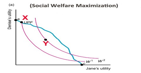
Social Welfare Maximization
The Simple Analystics of “Welfare Maximisation” has presented a more thorough and systematic analysis of the problem of social welfare maximisation. It is a summary of the static long-run general equilibrium conditions of a perfectly competitive economy.
It combines the Pareto optimality conditions with the social welfare function and provides a determinate and unique solution to the problem of maximisation of social welfare.
The social welfare function, which customarily consists of the benefit function of consumers and cost function of real power generation, is modified to include the cost function of reactive power generation. This will incorporate an economic signal regarding production and consumption of reactive power within locational marginal prices payable to the suppliers and chargeable from the consumers at different locations. The reactive power cost function of a synchronous generator is modeled using the lost opportunity to trade real power to produce required amount of reactive power.
Assumptions of Maximization of Social Welfare:
- There are two homogeneous and perfectly divisible inputs, labour (L) and capital (K). The two are supplied in fixed quantities.
- Only two homogeneous goods, X and Y are produced in the economy. The production function for each good is given and does not change. Each production function is smooth, shows constant returns to scale and diminishing marginal rate of technical substitution along any isoquant which means that the isoquants are convex to the origin.
- The goal of consumers is utility maximisation and the goal of firms is profit maximisation.
- The production functions are independent. This rules out joint products and external economies and diseconomies in production.
- The utilities of consumers are independent. Bandwagon, snob and Veblen effects are ruled out. There are no external economies or diseconomies in consumption.
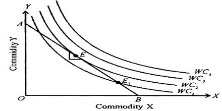
- There are two individuals, A and B, in the economy. Each has a set of smooth indifference curves convex to the origin which reflect consistent ordinal preference functions.
- There is a social welfare function that is based on the positions of A and B in their own preference scale, i.e. W = W (WA, WB). It presents a unique preference ordering of all possible situations,
Explanation to Maximization of Social Welfare:
- The input of labour into the production of X and Y,
- The input of capital into the production of X and Y;
- The total amount of X and Y produced; and
- The distribution of X and Y between the two individuals A and B.
From the Production Function to the Production Possibility Curve
The diagram describes the general equilibrium of production. There are fixed amounts of two inputs, labour (L) and Capital (K) available to the economy for the production of two commodities X and Y. Ox is the origin of input labour which is measured along the horizontal axis and Oy of input capital which is measured along the vertical axis. The horizontal sides of the two axes, Ox and Oy represent commodity X and the vertical sides commodity Y. The production function for each commodity is given by smooth Isoquants which are characterised by constant returns to scale and diminishing marginal rates of technical substitution MRTS. These Isoquants are X1, X2 and X3 for commodity X for which Ox is the origin and Y1, Y2 and Y3 for commodity Y for which Oy is the origin.
At points P1 Q1 and R1 an Isoquant of commodity X is tangent to an Isoquant of commodity Y and so satisfies the condition xMRTSLK = yMRTSLK. By joining these tangency points leads to the production contract curve Ox P1Q1R1Oy in input space. The various points on this contract curve are of efficiency locus where an increase in the production of X implies a necessary reduction in the output of Y.
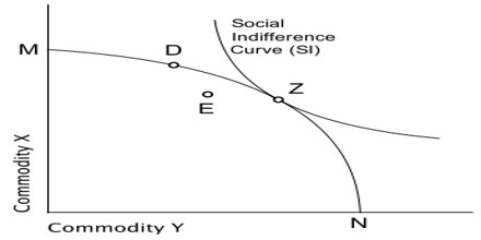
From this production contract curve, we can trace the production possibility curve or transformation curve in the output space from the input space. The production possibility curve associated with the contract curve OxP1Q1R1Oy of the diagram is plotted as TC. This curve shows the various combinations of X and Y that can be produced with fixed amounts of labour and capital. Consider point P1 on the contract curve and input space of diagram.
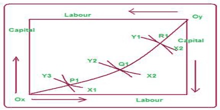
If the Isoquant Y3 represents 300 units of input Y and X1 and 50 units of X they are mapped in the output space as point P. Likewise points Q1 and R1of the diagram are traced in the output space as points Q and R respectively in the diagram. By joining points P, Q and R we derive the production possibility curve TC for commodity X and Y. With given amounts of labour an capital and fixed technology, the economy cannot attain any point above TC curve.
Nor can it have a point inside the TC curve for that will remain underutilisation of the two factor endowments. The economy must therefore be on the TC curve to maximise the community welfare. Further, the slope of any point on the production on the production possibility curve of diagram reflects the marginal rate of transformation MRT of X into Y. in other words, it indicates by how much the output of Y must be reduced by transferring enough capital and labour to produce one more unit of X.