Market equilibrium under the assumption that tastes and preferences of the consumers, prices of the related commodities, incomes of the consumers, technology, size of the market, prices of the inputs used in production, etc remain constant. However, with changes in one or more of these factors, either the supply or the demand curve or both may shift, thereby affecting the equilibrium price and quantity.
Demand Shift
Consider in which we depict the impact of demand shift when the number of firms is fixed. Here, the initial equilibrium point is E where the market demand curve DD0 and the market supply curve SS0 intersect so that q0 and p0 are the equilibrium quantity and price respectively.
Now suppose the market demand curve shifts rightward to DD2 with supply curve remaining unchanged at SS0, as shown in panel (a). This shift indicates that at any price the quantity demanded is more than before. Therefore, at price p0 now there is excess demand in the market equal to q q” 0 0 . In response to this excess demand some individuals will be willing to pay higher price and the price would tend to rise. The new equilibrium is attained at G where the equilibrium quantity q2 is greater than q0 and the equilibrium price p2 is greater than p0.
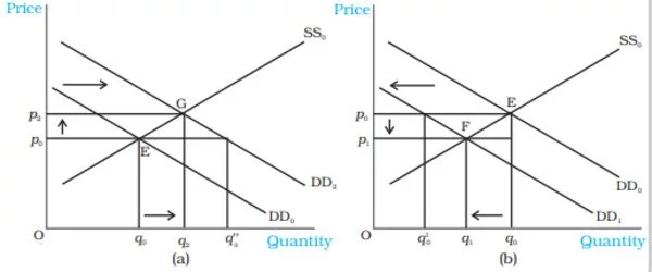
Similarly if the demand curve shifts leftward to DD1, as shown in panel (b), at any price the quantity demanded will be less than what it was before the shift. Therefore, at the initial equilibrium price p0 now there will be excess supply in the market equal to q’ q0 0 in response to which some firms will reduce the price of their commodity so that they can sell their desired quantity. The new equilibrium is attained at the point F at which the demand curve DD1 and the supply curve SS0 intersect and the resulting equilibrium price p1 is less than p0 and quantity q1 is less than q0. Notice that the direction of change in equilibrium price and quantity is same whenever there is a shift in demand curve.
Having developed the general theory, we now consider some examples to understand how demand curve and the equilibrium quantity and price are affected in response to a change in some of the aforementioned factors which are also enlisted in Chapter 2. More specifically, we would analyze the impact of increase in consumers’ income and an increase in the number of consumers on equilibrium.
Suppose due to a hike in the salaries of the consumers, their incomes increase. How would it affect equilibrium? With an increase in income, consumers are able to spend more money on some goods. The consumers will spend less on an inferior good with increase in income whereas for a normal good, with prices of all commodities and tastes and preferences of the consumers held constant, we would expect the demand for the good to increase at each price as a result of which the market demand curve will shift rightward. Here we consider the example of a normal good like clothes, the demand for which increases with an increase in the income of consumers, thereby causing a rightward shift in the demand curve. However, this income increase does not have any impact on the supply curve, which shifts only due to some changes in the factors relating to technology or cost of production of the firms. Thus, the supply curve remains unchanged. In Figure (a), this is shown by a shift in the demand curve from DD0 to DD2 but the supply curve remains unchanged at SS0. From the figure, it is clear that at the new equilibrium, the price of clothes is higher and the quantity demanded and sold is also higher.
Now let us turn to another example. Suppose due to some reason, there is increase in the number of consumers in the market for clothes. As the number of consumers increases, other factors remaining unchanged, at each price, more clothes will be demanded. Thus, the demand curve will shift rightwards. But this increase in the number of consumers does not have any impact on the supply curve since the supply curve may shift only due to changes in the parameters relating to firms’ behavior or with an increase in the number of firms. This case again can be illustrated through Figure (a) in which the demand curve DD0 shifts rightward to DD2, the supply curve remaining unchanged at SS0. The figure clearly shows that compared to the old equilibrium point E, at point G which is the new equilibrium point, there is an increase in both price and quantity demanded and supplied.
Supply Shift
In Figure, we show the impact of a shift in supply curve on the equilibrium price and quantity. Suppose, initially, the market is in equilibrium at point E where the market demand curve DD0 intersects the market supply curve SS0 such that the equilibrium price is p0 and the equilibrium quantity is q0.
Now, suppose due to some reason, the market supply curve shifts leftward to SS2 with the demand curve remaining unchanged, as shown in panel (a). Because of the shift, at the prevailing price, p0, there will be excess demand equal to q” 0 qo in the market. Some consumers who are unable to obtain the good will be willing to pay higher prices and the market price tends to increase. The new equilibrium is attained at point G where the supply curve SS2 intersects the demand curve DD0 such that q2 quantity will be bought and sold at price p2. Similarly, when supply curve shifts rightward, as shown in panel (b), at p0 there will be supply excess of goods equal to q0 q’0 . In response to this excess supply, some firms will reduce their price and the new equilibrium will be attained at F where the supply curve SS1 intersects the demand curve DD0 such that the new market price is p1 at which q1 quantity is bought and sold.Notice the directions of change in price and quantity are opposite whenever there is a shift in supply curve.
Now with this understanding, we can analyse the behaviour of equilibrium price and quantity when various aspects of the market change. Here, we will consider the effect of an increase in input price and an increase in number of firms on equilibrium.
Let us consider a situation where all other things remaining constant, there is an increase in the price of an input used in the production of a commodity. This will increase the marginal cost of production of the firms using this input. Therefore, at each price, the market supply will be less than before. Hence, the supply curve shifts leftward. In the Figure (a), this is shown by a shift in the supply curve from SS0 to SS2. But this increase in input price has no impact on the demand of the consumers since it does not depend on the input prices directly. Therefore, the demand curve remains unchanged. In Figure (a), this is shown by the demand curve remaining unchanged at DD0. As a result, compared to the old equilibrium, now the market price rises, and the quantity produced decreases.