Data Mining
Data mining is a powerful new technology with great potential to help companies focus on the most important information in the data they have collected about the behavior of their customers and potential customers. It discovers information within the data that queries and reports can’t effectively reveal.
Generally, data mining is the process of analyzing data from different perspectives and summarizing it into useful information – information that can be used to increase revenue, cuts costs, or both. Data mining software is one of a number of analytical tools for analyzing data. It allows users to analyze data from many different dimensions or angles, categorize it, and summarize the relationships identified. Technically, data mining is the process of finding correlations or patterns among dozens of fields in large relational databases.
It discovers information within the data that queries and reports can’t effectively reveal.
Some samples:
* Internet e-Commerce
* Direct Marketing
* Healthcare
* Genetics
* CRM
* Telecommunications
* Utilities
*Financial Services
Data: Data are any facts, numbers, or text that can be processed by a computer. Today, organizations are accumulating vast and growing amounts of data in different formats and different databases. This includes:
operational or transactional data such as, sales, cost, inventory, payroll, and accounting
no operational data, such as industry sales, forecast data, and macro economic data
meta data – data about the data itself, such as logical database design or data dictionary definitions
Information: The patterns, associations, or relationships among all this data can provide information. For example, analysis of retail point of sale transaction data can yield information on which products are selling and when.
Knowledge: Information can be converted into knowledge about historical patterns and future trends. For example, summary information on retail supermarket sales can be analyzed in light of promotional efforts to provide knowledge of consumer buying behavior. Thus, a manufacturer or retailer could determine which items are most susceptible to promotional efforts.
What can data mining do: Companies with a strong consumer focus – retail, financial, communication, and marketing organizations, primarily use Data mining today. It enables these companies to determine relationships among “internal” factors such as price, product positioning, or staff skills, and “external” factors such as economic indicators, competition, and customer demographics. And, it enables them to determine the impact on sales, customer satisfaction, and corporate profits. Finally, it enables them to “drill down” into summary information to view detail transactional data. With data mining, a retailer could use point-of-sale records of customer purchases to send targeted promotions based on an individual’s purchase history. By mining demographic data from comment or warranty cards, the retailer could develop products and promotions to appeal to specific customer segments.
Example: Blockbuster Entertainment mines its video rental history database to recommend rentals to individual customers. American Express can suggest products to its cardholders based on analysis of their monthly expenditures.
WalMart is pioneering massive data mining to transform its supplier relationships. WalMart captures point-of-sale transactions from over 2,900 stores in 6 countries and continuously transmits this data to its massive 7.5 terabyte Teradata data warehouse. WalMart allows more than 3,500 suppliers, to access data on their products and perform data analyses. These suppliers use this data to identify customer buying patterns at the store display level. They use this information to manage local store inventory and identify new merchandising opportunities. In 1995, WalMart computers processed over 1 million complex data queries.
The National Basketball Association (NBA) is exploring a data mining application that can be used in conjunction with image recordings of basketball games. The Advanced Scout software analyzes the movements of players to help coaches orchestrate plays and strategies. For example, an analysis of the play-by-play sheet of the game played between the New York Knicks and the Cleveland Cavaliers on January 6, 1995 reveals that when Mark Price played the Guard position, John Williams attempted four jump shots and made each one! Advanced Scout not only finds this pattern, but explains that it is interesting because it differs considerably from the average shooting percentage of 49.30% for the Cavaliers during that game.
By using the NBA universal clock, a coach can automatically bring up the video clips showing each of the jump shots attempted by Williams with Price on the floor, without needing to comb through hours of video footage. Those clips show a very successful pick-and-roll play in which Price draws the Knick’s defense and then finds Williams for an open jump shot.
How does data mining work: While large-scale information technology has been evolving separate transaction and analytical systems, data mining provides the link between the two. Data mining software analyzes relationships and patterns in stored transaction data based on open-ended user queries. Several types of analytical software are available: statistical, machine learning, and neural networks.
Data mining consists of five major elements:
Extract, transform, and load transaction data onto the data warehouse system.
Store and manage the data in a multidimensional database system.
Provide data access to business analysts and information technology professionals.
Analyze the data by application software.
Present the data in a useful format, such as a graph or table.
Different levels of analysis are available:
Artificial neural networks: Non-linear predictive models that learn through training and resemble biological neural networks in structure.
Genetic algorithms: Optimization techniques that use processes such as genetic combination, mutation, and natural selection in a design based on the concepts of natural evolution.
Decision trees: Tree-shaped structures that represent sets of decisions. These decisions generate rules for the classification of a dataset. Specific decision tree methods include Classification and Regression Trees (CART) and Chi Square Automatic Interaction Detection (CHAID) . CART and CHAID are decision tree techniques used for classification of a dataset. They provide a set of rules that you can apply to a new (unclassified) dataset to predict which records will have a given outcome. CART segments a dataset by creating 2-way splits while CHAID segments using chi square tests to create multi-way splits. CART typically requires less data preparation than CHAID.
Nearest neighbor method: A technique that classifies each record in a dataset based on a combination of the classes of the k record(s) most similar to it in a historical dataset (where k 1). Sometimes called the k-nearest neighbor technique.
Rule induction: The extraction of useful if-then rules from data based on statistical significance.
Data visualization: The visual interpretation of complex relationships in multidimensional data. Graphics tools are used to illustrate data relationships.
Neural network method of data mining is described bellow:
Neural Networks: When data mining algorithms are talked about these days most of the time people are talking about either decision trees or neural networks. Of the two neural networks have probably been of greater interest through the formative stages of data mining technology. As we will see neural networks do have disadvantages that can be limiting in their ease of use and ease of deployment, but they do also have some significant advantages. Foremost among these advantages is their highly accurate predictive models that can be applied across a large number of different types of problems.
To be more precise with the term “neural network” one might better speak of an “artificial neural network”. True neural networks are biological systems (a k a brains) that detect patterns, make predictions and learn. The artificial ones are computer programs implementing sophisticated pattern detection and machine learning algorithms on a computer to build predictive models from large historical databases. Artificial neural networks derive their name from their historical development which started off with the premise that machines could be made to “think” if scientists found ways to mimic the structure and functioning of the human brain on the computer. Thus historically neural networks grew out of the community of Artificial Intelligence rather than from the discipline of statistics. Despite the fact that scientists are still far from understanding the human brain let alone mimicking it, neural networks that run on computers can do some of the things that people can do.
It is difficult to say exactly when the first “neural network” on a computer was built. During World War II a seminal paper was published by McCulloch and Pitts which first outlined the idea that simple processing units (like the individual neurons in the human brain) could be connected together in large networks to create a system that could solve difficult problems and display behavior that was much more complex than the simple pieces that made it up. Since that time much progress has been made in finding ways to apply artificial neural networks to real world prediction problems and in improving the performance of the algorithm in general. In many respects the greatest breakthroughs in neural networks in recent years have been in their application to more mundane real world problems like customer response prediction or fraud detection rather than the loftier goals that were originally set out for the techniques such as overall human learning and computer speech and image understanding.
Applying Neural Networks to Business: Neural networks are very powerful predictive modeling techniques but some of the power comes at the expense of ease of use and ease of deployment. As we will see in this section, neural networks, create very complex models that are almost always impossible to fully understand even by experts. The model itself is represented by numeric values in a complex calculation that requires all of the predictor values to be in the form of a number. The output of the neural network is also numeric and needs to be translated if the actual prediction value is categorical (e.g. predicting the demand for blue, white or black jeans for a clothing manufacturer requires that the redictor values blue, black and white for the predictor color to be converted to numbers).
Because of the complexity of these techniques much effort has been expended in trying to increase the clarity with which the model can be understood by the end user. These efforts are still in there infancy but are of tremendous importance since most data mining techniques including neural networks are being deployed against real business problems where significant investments are made based on the predictions from the models (e.g. consider trusting the predictive model from a neural network that dictates which one million customers will receive a $1 mailing).
Where to Use Neural Networks: Neural networks are used in a wide variety of applications. They have been used in all facets of business from detecting the fraudulent use of credit cards and credit risk prediction to increasing the hit rate of targeted mailings. They also have a long history of application in other areas such as the military for the automated driving of an unmanned vehicle at 30 miles per hour on paved roads to biological simulations such as learning the correct pronunciation of English words from written text.
What does a neural net look like: A neural network is loosely based on how some people believe that the human brain is organized and how it learns. Given that there are two main structures of consequence in the neural network:
The node – which loosely corresponds to the neuron in the human brain.
The link – which loosely corresponds to the connections between neurons (axons, dendrites and synapses) in the human brain.
In Figure 2.3 there is a drawing of a simple neural network. The round circles represent the nodes and the connecting lines represent the links. The neural network functions by accepting predictor values at the left and performing calculations on those values to produce new values in the node at the far right. The value at this node represents the prediction from the neural network model. In this case the network takes in values for predictors for age and income and predicts whether the person will default on a bank loan.
Figure 2.3 A simplified view of a neural network for prediction of loan default.
How does a neural net make a prediction: In order to make a prediction the neural network accepts the values for the predictors on what are called the input nodes. These become the values for those nodes those values are then multiplied by values that are stored in the links (sometimes called links and in some ways similar to the weights that were applied to predictors in the nearest neighbor method). These values are then added together at the node at the far right (the output node) a special thresholding function is applied and the resulting number is the prediction. In this case if the resulting number is 0 the record is considered to be a good credit risk (no default) if the number is 1 the record is considered to be a bad credit risk (likely default).
A simplified version of the calculations made in Figure 2.3 might look like what is shown in Figure 2.4. Here the value age of 47 is normalized to fall between 0.0 and 1.0 and has the value 0.47 and the income is normalized to the value 0.65. This simplified neural network makes the prediction of no default for a 47-year-old making $65,000. The links are weighted at 0.7 and 0.1 and the resulting value after multiplying the node values by the link weights is 0.39. The network has been trained to learn that an output value of 1.0 indicates default and that 0.0 indicates non-default. The output value calculated here (0.39) is closer to 0.0 than to 1.0 so the record is assigned a non-default prediction.
Figure 2.4 The normalized input values are multiplied by the link weights and added together at the output.
How is the neural net model created:
The neural network model is created by presenting it with many examples of the predictor values from records in the training set (in this example age and income are used) and the prediction value from those same records. By comparing the correct answer obtained from the training record and the predicted answer from the neural network it is possible to slowly change the behavior of the neural network by changing the values of the link weights. In some ways this is like having a grade school teacher ask questions of her student (a.k.a. the neural network) and if the answer is wrong to verbally correct the student. The greater the error the harsher the verbal correction. So that large errors are given greater attention at correction than are small errors.
For the actual neural network it is the weights of the links that actually control the prediction value for a given record. Thus the particular model that is being found by the neural network is in fact fully determined by the weights and the architectural structure of the network. For this reason it is the link weights that are modified each time an error is made.
How complex can the neural network model become?
The models shown in the figures above have been designed to be as simple as possible in order to make them understandable. In practice no networks are as simple as these. Networks with many more links and many more nodes are possible. This was the case in the architecture of a neural network system called NETtalk that learned how to pronounce written English words. Each node in this network was connected to every node in the level above it and below it resulting in 18,629 link weights that needed to be learned in the network.
In this network there was a row of nodes in between the input nodes and the output nodes. These are called hidden nodes or the hidden layer because the values of these nodes are not visible to the end user the way that the output nodes are (that contain the prediction) and the input nodes (which just contain the predictor values). There are even more complex neural network architectures that have more than one hidden layer. In practice one hidden layer seems to suffice however.
The learning that goes on in the hidden nodes.
The learning procedure for the neural network has been defined to work for the weights in the links connecting the hidden layer. A good metaphor for how this works is to think of a military operation in some war where there are many layers of command with a general ultimately responsible for making the decisions on where to advance and where to retreat. The general probably has several lieutenant generals advising him and each lieutenant general probably has several major generals advising him. This hierarchy continuing downward through colonels and privates at the bottom of the hierarchy.
This is not too far from the structure of a neural network with several hidden layers and one output node. You can think of the inputs coming from the hidden nodes as advice. The link weight corresponds to the trust that the general has in his advisors. Some trusted advisors have very high weights and some advisors may no be trusted and in fact have negative weights. The other part of the advice from the advisors has to do with how competent the particular advisor is for a given situation. The general may have a trusted advisor but if that advisor has no expertise in aerial invasion and the question at hand has to do with a situation involving the air force this advisor may be very well trusted but the advisor himself may not have any strong opinion one way or another.
In this analogy the link weight of a neural network to an output unit is like the trust or confidence that a commander has in his advisors and the actual node value represents how strong an opinion this particular advisor has about this particular situation. To make a decision the general considers how trustworthy and valuable the advice is and how knowledgeable and confident each advisor is in making their suggestion and then taking all of this into account the general makes the decision to advance or retreat.
In the same way the output node will make a decision (a prediction) by taking into account all of the input from its advisors (the nodes connected to it). In the case of the neural network this decision is reach by multiplying the link weight by the output value of the node and summing these values across all nodes. If the prediction is incorrect the nodes that had the most influence on making the decision have their weights modified so that the wrong prediction is less likely to be made the next time.
This learning in the neural network is very similar to what happens when the wrong decision is made by the general. The confidence that the general has in all of those advisors that gave the wrong recommendation is decreased – and all the more so for those advisors who were very confident and vocal in their recommendation. On the other hand any advisors who were making the correct recommendation but whose input was not taken as seriously would be taken more seriously the next time. Likewise any advisor that was reprimanded for giving the wrong advice to the general would then go back to his advisors and determine which of them he had trusted more than he should have in making his recommendation and who he should have listened more closely to.
Method of using the model: Once a model has been created by a data mining application, the model can then be used to make predictions for new data. The process of using the model is distinct from the process that creates the model. Typically, a model is used multiple times after it is created to score different databases. For example, consider a model that has been created to predict the probability that a customer will purchase something from a catalog if it is sent to them. The model would be built by using historical data from customers and prospects that were sent catalogs, as well as information about what they bought (if anything) from the catalogs. During the model-building process, the data mining application would use information about the existing customers to build and validate the model. In the end, the result is a model that would take details about the customer (or prospects) as inputs and generate a number between 0 and 1 as the output. This process is illustrated below:
After a model has been created based on historical data, it can then be applied to new data in order to make predictions about unseen behavior. This is what data mining (and more generally, predictive modeling) is all about. The process of using a model to make predictions about behavior that has yet to happen is called “scoring.” The output of the model, the prediction, is called a score. Scores can take just about any form, from numbers to strings to entire data structures, but the most common scores are numbers (for example, the probability of responding to a particular promotional offer).
Scoring is the unglamorous workhorse of data mining. It doesn’t have the sexiness of a neural network or a genetic algorithm, but without it, data mining is pretty useless. (There are some data mining applications that cannot score the models that they produce — this is akin to building a house and forgetting to put in any doors.) At the end of the day, when your data mining tools have given you a great predictive model, there’s still a lot of work to be done. Scoring models against a database can be a time-consuming, error-prone activity, so the key is to make it part of a smoothly flowing process.
2. The Process
Scoring usually fits somewhere inside of a much larger process. In the case of one application of data mining, database marketing, it usually goes something like this:
1. The process begins with a database containing information about customers or prospects. This database might be part of a much larger data warehouse or it might be a smaller marketing data mart.
2. A marketing user identifies a segment of customers of interest in the customer database. A segment might be defined as “existing customers older than 65, with a balance greater than $1000 and no overdue payments in the last three months.” The records representing this customer segment might be siphoned off into a separate database table or the records might be identified by a piece of SQL that represents the desired customers.
3. The selected group of customers is then scored by using a predictive model. The model might have been created several months ago (at the request of the marketing department) in order to predict the customer’s likelihood of switching to a premium level of service. The score, a number between 0 and 1, represents the probability that the customer will indeed switch if they receive a brochure describing the new service in the mail. The scores are to be placed in a database table, with each record containing the customer ID and that customer’s numerical score.
4. After the scoring is complete, the customers then need to be sorted by their score value. The top 25% will be chosen to receive the premium service offer. A separate database table that contains the records for the top 25% of the scoring customers will be created.
5. After the customers with the top 25% of the scores are identified, the information necessary to send them the brochure (name and address) will need to be pulled out of the data warehouse and a tape created containing all of this information.
6. Finally, the tape will be shipped to a company (sometimes referred to as a “mail house”)where the actual mailing will occur.
The marketing department typically determines when and where the marketing campaigns take place. In past years, this process might be scheduled to happen once every six months, with large numbers of customers being targeted every time the marketing campaign is executed. Current thinking is to move this process into a more continuous schedule, whereby small groups of customers are targeted on a weekly or even daily basis.
The future of data mining:
In the short-term, the results of data mining will be in profitable, if mundane, business related areas. Micro-marketing campaigns will explore new niches. Advertising will target potential customers with new precision.
In the medium term, data mining may be as common and easy to use as e-mail. We may use these tools to find the best airfare to New York, root out a phone number of a long-lost classmate, or find the best prices on lawn mowers.
The long-term prospects are truly exciting. Imagine intelligent agents turned loose on medical research data or on sub-atomic particle data. Computers may reveal new treatments for diseases or new insights into the nature of the universe. There are potential dangers, though, as discussed below.