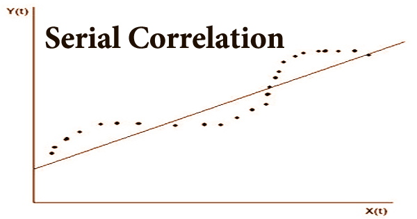
Serial correlation, also known as autocorrelation, is a statistical term that refers to the link between the present value of a variable and a lagged value of the same variable from previous time periods. It’s the similarity of observations as a function of the time lag between them, to put it another way. Financial analysts frequently utilize serial correlation, also known as autocorrelation, to forecast future price movements of a security, such as a stock, based on recent price movements.
When the level of a variable impacts its future level, serial correlation is common in repeating patterns. When error terms in a time series move from one period to the next, this is known as serial correlation. Serial correlation determines the relationship, if any, between the same variable measured over different periods of time. To put it another way, the mistake for one time period an is connected to the error for the next time period b.
Serial correlation is a statistical concept that is related to autocorrelation and lagged correlation. Autocorrelation analysis is a mathematical method for detecting recurring patterns, such as the presence of a periodic signal masked by noise or the identification of a signal’s missing fundamental frequency suggested by its harmonic frequencies. Technical analysts in finance utilize this correlation to assess how effectively the previous price of an investment predicts the future price.
If a security’s current value is shown to be serially linked with prior values, the correlation can be utilized to anticipate future values. Technical analysts verify a security’s or a set of securities’ lucrative trends and assess the risk associated with investing possibilities. Autocorrelation is defined variously in different fields of study, and not all of these definitions are comparable. In certain domains, the terms autocovariance and autocorrelation are interchangeable.
Financial analysts frequently employ serial correlations in the development of financial models in order to forecast the likely future values of a stock or other financial security. It’s a statistical term that refers to the association between observations of the same variable across time. There is no correlation if the serial correlation of a variable is 0, and each observation is independent of the others.
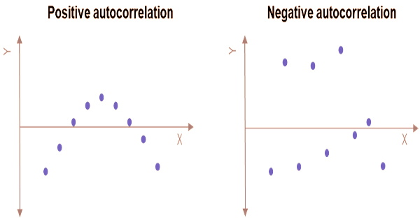
The Pearson correlation between the process’s values at various times, as a function of the two times or the time lag, is the autocorrelation of a real or complicated random process. Positive serial correlations indicate that values are likely to change in the same way, or direction, in future time periods as they have in recent past time periods; negative serial correlations indicate that values are likely to change in the opposite direction in future time periods as they have in recent past time periods.
If the serial correlation of a variable skews toward one, the observations are serially correlated, and future observations are influenced by previous values. In other words, a serially linked variable has a pattern and is not random. Mean aversion occurs when the current price of a security and the price of the security in a previous time period have a positive serial correlation.
When a model isn’t fully correct, it produces different results in real-world applications, which are known as error terms. The error term is serially correlated when error terms from various (typically contiguous) periods (or cross-section data) are correlated. Aversion to the mean means that price fluctuations in the asset are more likely to follow patterns and, over time, will have greater standard deviations than if there were no link. Normalizing the autocovariance function to get a time-dependent Pearson correlation coefficient is standard practice in several areas (e.g. statistics and time series analysis).
Normalization is generally abandoned in other areas (e.g., engineering), and the words “autocorrelation” and “autocovariance” are used interchangeably. Serial correlation can be measured using a number of sophisticated statistical formulae; nevertheless, most techniques compute serial correlation with values ranging from -1 to +1. In time-series research, serial correlation arises when mistakes from one period transfer over to subsequent periods. When projecting stock dividend growth, for example, an overestimate in one year will lead to overestimates in subsequent years.
There is no connection if the serial correlation value is 0. It was invented in engineering to assess how a signal, such as a computer signal or a radio wave, changes over time in comparison to itself. Economists and econometricians utilized the measure to evaluate economic data over time, and it rose in prominence in economic circles.
To put it another way, there is no discernible link or pattern between a variable’s present value and its value in prior time periods. Positive serial correlation is shown by numbers closer to +1, whereas negative serial correlation is indicated by values between zero and -1. The normalization is essential because the interpretation of the autocorrelation as a correlation gives a scale-free measure of the intensity of statistical dependence, and it affects the statistical characteristics of the calculated autocorrelations.
Furthermore, determining the correlation structure increases the realism of any model-based simulated time series. Investment techniques are less risky when accurate models are used. Serial correlation measurements can assist optimize returns on investment, minimize investment risk, or both by increasing the accuracy of financial models. The study of serial correlations did not begin in the financial services sector; instead, it began in the field of engineering.
Information Sources: