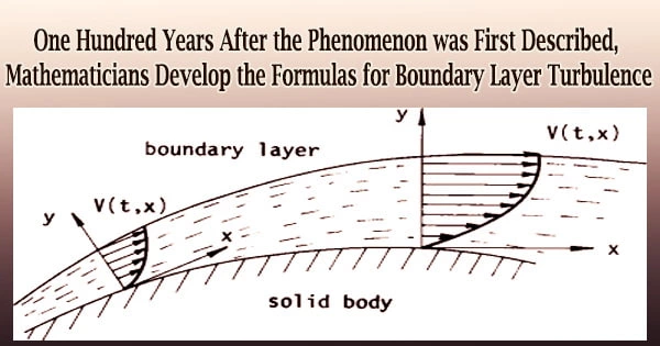
Many people feel unpleasant or even sick when there is turbulence. It has also caused headaches for researchers. For at least a century, mathematicians have been attempting to formulate the turbulence that results from a flow interacting with a boundary.
A thorough explanation of boundary layer turbulence has now been published by an international team of mathematicians, lead by professors Björn Birnir from UC Santa Barbara and Luiza Angheluta from the University of Oslo.
The article, which summarizes decades of research on the subject, is published in Physical Review Research. The theory combines into a mathematical formula the Navier-Stokes equation.
Theodore von Kármán, a Hungarian physicist, and Ludwig Prandtl, a German scientist, two giants of fluid dynamics, were the first to explain this phenomenon about 1920.
“They were honing in on what’s called boundary layer turbulence,” said Birnir, director of the Center for Complex and Nonlinear Science.
When a flow interacts with a boundary, such as the fluid’s surface, a pipe wall, the Earth’s surface, or another object, it creates turbulence.
Through experimentation, Prandtl discovered that he could separate the border layer into four unique areas based on their proximity to the boundary. The viscous layer develops just adjacent to the boundary, where the thickness of the flow dampens turbulence.
A transitional buffer region then followed the inertial region, where turbulence is most pronounced. According to a formula by von Kármán, the boundary layer flow is least impacted by the boundary in the wake.
However, the fluid’s velocity varies in a very precise way as it gets closer to the border. In the viscous and buffer layers, its average velocity rises, and in the inertial layer, it changes to a logarithmic function.
Researchers have struggled to explain and comprehend the origins of this “log law,” which Prandtl and von Kármán discovered.
I think, ultimately, we will be able to use this theory to understand both atmospheric turbulence and the jet stream. It’s going to be quite useful.
Professors Björn Birnir
Over the boundary layer, the flow’s fluctuation or departure from the mean velocity also exhibited odd behavior. The goal of the research was to comprehend these two factors and create formulas that might characterize them.
Albert Alan Townsend, an Australian mechanical engineer, postulated in the 1970s that boundary-attached eddies had an impact on the shape of the mean velocity curve. If accurate, it might explain both the physics underlying the log rule and the peculiar shape the curve assumes as it passes through the several layers, according to Birnir.
In 2010, University of Illinois mathematicians published a formal description of these linked eddies that included mathematics. The study also discussed how these eddies might channel energy away from the fluid border and into the surrounding fluid.
“There’s a whole hierarchy of eddies,” Birnir said.
The fact that the smaller eddies provide energy to the larger ones that extend all the way into the inertial layer can explain the log law.
Detached eddies, on the other hand, can move around inside a fluid and are equally crucial to boundary layer turbulence. Deriving a formal description of these was the main goal of Birnir and his co-authors.
“What we showed in this paper is that you need to include these detached eddies in the theory as well in order to get the exact shape of the mean velocity curve,” he said.
The mathematical formulation of the mean velocity and variation that Prandtl and von Kármán first wrote about over a century ago was developed by their team by combining all these ideas. They validated their findings by comparing their calculations to computer simulations and experimental data.
“Finally, there was a complete analytical model that explained the system,” Birnir said.
Engineers and scientists can change many parameters to predict the behavior of a fluid using this new mathematical framework. Additionally, boundary layer turbulence can be seen in a variety of industries, including transportation, meteorology, and more.
“I think it’s going to have a lot of applications,” Birnir remarked.
For instance, a thorough understanding of boundary turbulence can be used to create engines that are more effective, lessen pollution, and lower drag on many types of vehicles. A boundary flow can be used to simulate Earth’s atmosphere. The atmosphere is really just a thin layer of moving air that hugs the planet’s surface, despite its appearance of height.
“I think, ultimately, we will be able to use this theory to understand both atmospheric turbulence and the jet stream,” Birnir said. “It’s going to be quite useful.”
The significance of detached eddies in describing the turbulence shift in the buffer layer, in particular, shocked the authors. Understanding their behavior has started to shed light on other kinds of turbulence.
“In particular, we get insights into Lagrangian turbulence,” said Birnir, referencing the theory that describes turbulent behavior in reference fame that moves with the flow, like a raft on a river.
The Eulerian turbulence theory, in contrast, characterizes the fluid when it passes a fixed reference frame, such as a pier on a riverbank. Similar to how a river appears to vanish when you’re travelling downstream, attached eddies vanish in the moving reference frame.
“But the detached eddies are still there,” Birnir said, “and they seem to play a major role in Lagrangian turbulence.”
With these new tools which originated from studies on homogeneous turbulence, where there is no boundary the team is currently concentrating on investigating Lagrangian turbulence.
“Insights that you get in one field help you in another,” Birnir observed.