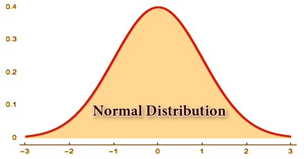
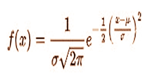
The most important distribution of probability in statistics is normal distribution, also called Gaussian or Gauss distribution since it suits many natural phenomena. In the natural and social sciences, distribution is commonly used. The Central Limit Theorem makes it important, stating that the averages obtained from independent, identically distributed random variables appear to form normal distributions irrespective of the type of distributions from which they are sampled. In statistical reports, from sample analysis and quality management to resource allocation, his familiar bell-shaped curve is ubiquitous. The general form of its density of probability function is
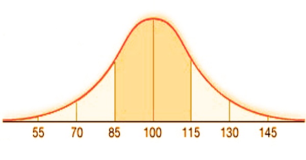
The boundary µ is the mean or assumption for the appropriation (and furthermore it’s middle and mode), while the boundary σ is its standard deviation. The fluctuation of the dispersion is σ2. An irregular variable with a Gaussian distribution is supposed to be regularly appropriated and is known as a typical stray. Two parameters define the graph of the normal distribution: the mean or average, which is the limit of the graph and the graph is always symmetrical; and the standard deviation, which defines the quantity of dispersion away from the mean. A small standard deviation (compared with the mean) produces a steep graph, while a flat graph is generated by a broad standard deviation (again compared to the mean).
Normal distributions are even, yet not all even circulations are ordinary. As a general rule, most valuing appropriations are not entirely typical. The two principal boundaries of a (typical) circulation are the mean and standard deviation. The boundaries decide the shape and probabilities of the dispersion. The state of the appropriation changes as the boundary esteems changes.
- Mean: As an indicator of central tendency, the mean is used by researchers. The distribution of variables calculated as ratios or intervals can be represented using it. The mean determines the position of the peak in a normal distribution graph, and most of the data points are clustered around the mean. Any adjustments made to the mean value would shift the curve along the X-axis, either to the left or right.
- Standard Deviation: The standard deviation calculates the dispersion, relative to the mean, of the data points. It defines how far the data points are located away from the mean and the distance between the mean and the observations is reflected.
On the chart, the standard deviation decides the width of the bend, and it fixes or extends the width of the circulation along the x-axis. Normally, a little standard deviation comparative with the mean creates a precarious bend, while an enormous standard deviation comparative with the mean delivers a compliment bend. There are two parameters of the standard normal distribution: the mean and the standard deviation. 68% of the observations are within +/- one standard deviation of the mean for a normal distribution, 95% are within +/- two standard deviations, and 99.7% are within +- three standard deviations.
By the normal density function, the normal distribution is provided, p(x)= e−(x−μ)2/2σ2/σ√2π. The constant 2.71828 in this exponential function is e, the mean, and σ is the standard deviation. The probability of a random variable falling within any given range of values is equal to the proportion between the given values and above the x-axis of the region enclosed under the function’s graph. Since the denominator (σ√2π), known as the normalizing coefficient, causes the absolute zone encased by the chart to be actually equivalent to solidarity, probabilities can be gotten straightforwardly from the relating region i.e., a region of 0.5 compares to a likelihood of 0.5.
Often, regular distribution is confused with the symmetrical distribution. Symmetrical distribution is one in which two mirror images are formed by a dividing line, but in addition to the bell curve showing a regular distribution, the actual data may be two humps or a series of hills. All forms of the (normal) distribution share the following characteristics:
- It is symmetric: With a perfectly symmetrical form, a normal distribution arrives. This implies that in the center, the distribution curve can be broken to create two equal halves. When one-half of the observations fall on either side of the curve, the symmetric form exists.
- The mean, median, and mode are equal: The center purpose of a normal distribution is the point with the greatest recurrence, which implies that it has the most perceptions of the variable. The midpoint is likewise where these three estimates fall. The measures are generally equivalent in an impeccably (typical) conveyance.
- Empirical rule: There is a constant proportion of the distance lying under the curve between the mean and the specific number of standard deviations from the mean in normally distributed results. For instance, 68.25% of all instances fall within +/- one standard deviation from the mean. 95% of all instances fall within +/- two regular deviations from the mean, while 99% of all instances fall within +/- three standard deviations from the mean.
- Skewness and kurtosis: The coefficients of skewness and kurtosis measure how different distribution is from a normal distribution. The symmetry of a normal distribution is determined by skewness, while kurtosis tests the thickness of the tail ends compared to the tails of a normal distribution.
Besides, Gaussian distribution has some remarkable properties that are significant in insightful investigations. For example, any direct blend of a fixed assortment of typical veers off is an ordinary stray. When the related variables are normally distributed, many results and techniques, such as propagation of uncertainty and least square parameter fitting, can be derived analytically in an explicit manner. The normal distribution is symmetrical and has zero skewness. In the event that the distribution of an informational collection has a skewness under nothing, or negative skewness, at that point the left tail of the dispersion is longer than the correct tail; positive skewness infers that the correct tail of the dissemination is longer than the left.
The term “Gaussian distribution” refers to the German mathematician Carl Friedrich Gauss, who, in connection with studies of astronomical observation errors, first developed a two-parameter exponential function in 1809. This research led Gauss to formulate his law of empirical error and to advance the principle of the approximation system of least squares. Most statisticians give credit for the discovery of normal distributions to the French scientist Abraham de Moivre. Moivre noted in the second edition of “The Doctrine of Chances,” that probabilities associated with random variables discreetly generated could be approximated by measuring the region under the exponential function graph. The British physicist James Clerk Maxwell, who formulated his law of distribution of molecular velocities in 1859, later generalized as the Maxwell-Boltzmann distribution law, was another prominent early application of normal distribution.
Information Sources: