Preface
Being a student of B.Ed. (Hons) at Institute of Education and Research, I went through a course named Practicum where I have completed a six month internship as trainee teacher at Engineering University Higher Secondary School. I took two classes each day- Social Science of class six (A) and Social Science of class Seven (B). During my role as a teacher I executed some tests for both the classes to determine the pupils’ common trend, their individual strengths and weaknesses and to give feedback and to fulfill my practicum requirements as well.
1. Statistical analysis
Statistical analysis of any particular test & test scores means the collection, presentation and analysis of those test & test scores with meaningful explanation and decision from that analysis.
Statistical analysis includes some specific and systematic steps, methods and measurement.
Here are some short descriptions about those:
1.1 Item Specification Table
Item specification table is used to determine the degree of pupils’ achieved desirable behavioral change. It is prepared before the execution of evaluation activity basing on the importance of content and learning objectives in terms of behavioral domains. This work plan is done in order to prepare items of the test.
1.2 Item analysis
Item analysis is done in order to determine the difficulty level, discrimination power and effectiveness of destructors of the test items, especially of the objective test items.
1.3 Frequency Distribution
It is difficult to make sense out of ungrouped data until they have been arranged or classified in some systematic way. Frequency distribution helps to classify or sort ungrouped data in a systematic way according to the frequency. It enables the researcher to make the data meaningful.
1.4 Range
Range is the difference between the highest and the lowest scores.
1.5 Class Interval
The scores have to be arranged in some small groups. The distance or difference of such a class is called class interval.
# Number of the class = (Range/class Interval) +1
1.6 Tabulation of scores
This is done in two steps. The first one is totally the scores in their proper intervals and the second one is to count the tallies and find out the frequency of each class interval. The sum of the frequencies is called N.
1.7 Mid Point of the Class Interval
# Mid Point = Lower limit of the class+(upper limit of the class -lower limit of the class)/2
1.8 Measures of Central Tendency
Measures of central tendency give the researcher a convenient if describing a set of data with a single number. The number resulting from computation of a measure of central tendency represents the average or typical score attained by a group of subjects. Measures of central tendencies are:
1.8.1 Mean
The mean is the arithmetic average of the scores and is the most frequently used measure of central tendency.
# True Mean = A.M.+(Σfd/N)i
| A.M.= Assumed Mean f = Frequency d = Deviation from the class Interval containing Assumed Mean Σfd = Summation of the products of f and d N = Total frequency i = Interval length |
1.8.2 Median
The median is that point in a distribution above and below which are 50% of the scores; in other words, the median is the midpoint.
# Median = L+{(N/2-cfu)/fm}i
| L = Lower point of the median class Cfu = Cumulative frequency of the class below the median class fm = Frequency of the median class i = Interval length N = Total frequency |
1.8.3 Mode
The mode is the score that is attained by more subjects than any other score.
# Mode = 3 median – 2 mean
2.0 Test and Examination – Explanation of the situation
- To fulfill my practicum requirement, I had to execute a 50-mark essay type test and a 50 mark MCQ test. But school authority did not allow me to take a two-hour or of more duration test. So I had to take the 50-mark essay type test in 3 parts:
Essay Type Test
Class Test no | Date | Major Subject | Syllabus | Duration | Total Marks |
1 | 17/03/07 | Geography | The Africa continent, Bangladesh | 30 Min | 20 |
2 | 02/04/07 | Population Education | Current situation of World Population | 25 Min | 15 |
3 | 16/04/07 | Economics | Three fundamental of Economics | 25 Min | 15 |
80 Min | 50 |
In this report I shall present this four sub tests as one combined essay type test of 50-marks and name it as Test – 1. Test results will follow the same procedure.
- On 03/11/05 I took the MCQ test of 50 marks which had the duration of 30 minutes, not 50 minutes because it was a tick method MCQ. This test will be named as Test – 2
- Syllabus of the MCQ test was the combined of whole syllabus.
- Mostly I had to teach geography, population education and Disaster as a joined their at September month.
3.0 Test Analysis
3.1. Analysis of Test-1 (Essay type Test)
3.1.1 General considerations
In preparing the essay type test, understated matters have been tried to maintain:
- 1. It is a 50-mark test. Total item no. is 6.
- The duration of the test is 80 minutes. Time per mark is 1.6 minute.
- The test has been constructed with both short essay type and broad essays in order to cover more areas of the content.
- Optional questions are not given.
- Number distribution was shown so that the students can prepare their answers according to the number distribution.
3.1.2 Subject wise Distribution
Integrated Social Science has been designed including major seven subjects:
- Sociology
- History
- Geography
- Political Science
- Economics
- Population Education
But sociology, history, Political Science and economics were not included for final exam. So, I had to teach and take tests without those subjects.
The essay type test has included all other subjects. Subject wise number distribution is shown below:
Subject | Distributed Marks | Percentage (%) |
| Geography | 20 | 40 |
| Population Edn. | 15 | 30 |
| Economics | 15 | 30 |
50 | 100 |
3.1.3 Item Specification
The item specification according to the domains of objectives of the essay type test is shown here:
Objective | Knowledge | Comprehension | Application | Analysis | Synthesis | Evaluation | Total marks |
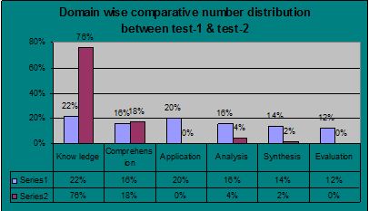
Percentage | 22% | 16% | 20% | 16% | 14% | 12% | |
| Marks | Marks | Marks | Marks | Marks | Marks | |
Geography | 5 | 1 | 0 | 8 | 0 | 6 | 20 |
Population Education | 3 | 5 | 0 | 0 | 7 | 0 | 15 |
Economics | 3 | 2 | 10 | 0 | 0 | 0 | 15 |
Total | 11 | 8 | 10 | 8 | 7 | 6 | 50 |
Comment
A good test covers all the domains of learning such as knowledge, comprehension, application, analysis, synthesis, and evaluation. This test fulfills this requirement covering all the domains of learning. A test should not be too easy or too difficult. 22% number has been given from knowledge sub-domain; items have also been taken from higher sub-domains such synthesis, evaluation, etc. It has been done in order to over all learning domains as well. But the test has a limitation. Usually the higher level of domain is lower the mark is distributed for the domain. This test couldn’t follow this rule properly. For example: 6 marks have been distributed for evaluation sub-domain, whereas 11 marks were given for knowledge 10 marks to assess application power. This irrelevancy can also be observed in analysis and synthesis sub-domains. Another factor is each subject area couldn’t cover every domains of learning. That was done consciously. Otherwise the test would be too much difficult. Students of class six don’t achieve much analysis, synthesis and evaluation power. So those domains were given less emphasis.
Reliability can be measured following the ‘Kuder and Richardson Method’.
3.1.4 Graphic presentation of Test – 1 analysis
Subject wise comparative number distribution
3.2. Analysis of Test-2 (MCQ Test)
3.2.1 General considerations
In preparing the Multiple Choice Questions (MCQ), understated matters have been tried to maintain:
- It is a 50-mark test. Total item no. is 50.Mark per item is 1. The duration of the test is 30 minutes. Time for each item is 36 seconds. Students were required to give tick mark (√) on the correct answer.50 minutes is not given as it was not a circle fill up test. So less time was required. All 36 seconds could be used for thinking.
- Four distractors are given for each item. Only one is correct answer.
- To make guessing difficult, distractors of a specific item are similar in length; no specific distractor is too lengthy than others, nor it is too short.
- The correct answers are arranged in a way so that students can’t guess it from the arrangement. For example: among 50 items, a total of 13 correct answers was arranged in distractor (Ka), 14 from distractor (kha), 12 from distractor (Ga),10 from distractor (Gha). And the correct answers is not arranged serially, rather it is random. So it was difficult to answer correctly basing on guess.
- Distractors of a specific item are plausible and homogeneous, not heterogeneous automatically eliminated.
- ‘All of the above’, ‘None of the above’-this type of distractors is only one item given. These distractors weaken the test.
- Negative sense distractors have been avoided.
- Stems and distractors have been clearly written so that it could make clear sense and avoid misconception.
- Unnecessary repetition of words in distractors has been avoided.
- Unfamiliar words are not used.
- MCQ is prepared from whole syllabus.
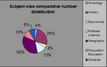
3.2.2 Subject wise Distribution
The MCQ test has included all the subjects. Subject wise number distribution is shown below:
Subject | Subject range | Distributed Marks | Percentage (%) |
| Sociology | 20 pages | 2 | 4 |
| History | 45 pages | 13 | 26 |
| Political science | 13 pages | 6 | 12 |
| Economics | 5 pages | 2 | 4 |
| Geography | 32 pages | 18 | 36 |
| Population Edn. | 7 pages | 5 | 10 |
| Disasters | 6 pages | 4 | 8 |
31 pages | 50 | 100 |
Comment
Distribution of marks differed because of the difference of ranges among the subjects. I have teach geography mainly and History after completing the whole syllabus, so emphasis on those chapters.
3.2.3 Item Specification
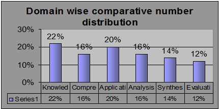
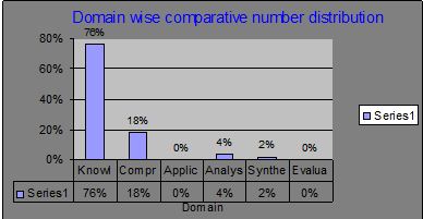
The item specification according to the domains of objectives of the MCQ test is shown below:
Objective | Knowledge | Comprehension | Application | Analysis | Synthesis | Evaluation | Total marks |
Percentage | 76% | 18% | 0% | 4% | 2% | 0% | |
| Marks | Marks | Marks | Marks | Marks | Marks | |
Sociology | 1 | 1 | 0 | 0 | 0 | 0 | 2 |
History | 13 | 0 | 0 | 0 | 0 | 0 | 13 |
Economics | 1 | 1 | 0 | 0 | 0 | 0 | 2 |
Political science | 3 | 3 | 0 | 0 | 0 | 0 | 6 |
Geography | 16 | 2 | 0 | 0 | 0 | 0 | 18 |
Population Education | 2 | 1 | 0 | 1 | 1 | 0 | 5 |
Disaster | 2 | 1 | 0 | 1 | 0 | 0 | 4 |
Total | 38 | 9 | 0 | 2 | 1 | 0 | 50 |
Comment
A good test covers all the domains of learning such as knowledge, comprehension, application, analysis, synthesis, and evaluation. This test could not fulfill that requirement of covering all the domains of learning. Actually it is too difficult to maintain domain wise questing in MCQ test specially when it is constructed for younger students. A test should not be too easy or too difficult. In this regard, 76% items has been given from knowledge sub-domain; items have also been taken from higher sub-domains such comprehension, analysis, synthesis, etc. It has been done in order to make the test neither too easy nor too difficult and to cover all learning domains as well. But the test has a limitation. Usually the higher level of domain is lower even no mark is distributed for the domain. This test couldn’t follow this rule properly. For example: 1 mark has been distributed for synthesis sub-domain, wheras no mark given to assess application and evaluation power. As a test maker I feel this quite difficult to prepare an MCQ test covering all the criterias. This can make the test too much difficult, especially for the students who have always faced traditional knowledge based tests and increase their exam fearness. Fully standardized test can be applied to them step-by-step and only after providing proper learning situations.
3.2.4 Graphic presentation of Test – 2 analysis
Subject wise comparative number distribution
Domain wise comparative number distribution
3.3 Graphic comparison between Test-1 and test-2
4.0 Test Result Analysis
4.1 Analysis of Test-1 results (Essay type test)
Student’s score in Test-1
Total student number of the class is 42. But on days of examination class was combined with B section. Here, to make a decent analysis and comparison, only the scores of the students were given who attended in all essay type and MCQ test. Total 50 students attended in the exam.
Scores 0f Test-1
Roll No. | Obtained Mark (Out of 50) | Roll No. | Obtained Mark (Out of 50) |
01 | 39 | 29 | 10 |
02 | 35 | 30 | 19.5 |
03 | 36 | 31 | 11.5 |
04 | 15 | 32 | 13 |
05 | 22 | 33 | 24.5 |
06 | 11 | 35 | 17 |
07 | 11 | 36 | 16 |
08 | 22 | 38 | 22 |
09 | 16 | 39 | 12 |
10 | 14.5 | 40 | 17.5 |
12 | 16.5 | 41 | 13.5 |
13 | 24 | 42 | 16 |
14 | 13 | 43 | 24 |
15 | 11.5 | 44 | 10 |
16 | 15 | 45 | 12.5 |
17 | 11.5 | 46 | 13 |
18 | 11.5 | 47 | 17.5 |
19 | 22 | 48 | 14 |
21 | 15 | 49 | 16 |
22 | 13.5 | 50 | 12.5 |
23 | 9.5 | 51 | 8 |
24 | 12.5 | 52 | 19 |
25 | 22.5 | 53 | 11 |
26 | 16 | 54 | 12 |
27 | 16.5 | N=50 | |
28 | 13 | ||
Tabulation of scores
# Number of the class = (Range/class Interval) +1
= {(Highest score-Lowest score)/Class Interval}+1
= {(39 – 8)/5}+1
= (31/5)+1
= 6.2 + 1
= 7.2
= 7 ( in full number)
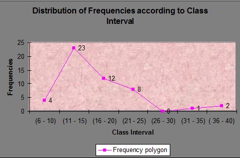
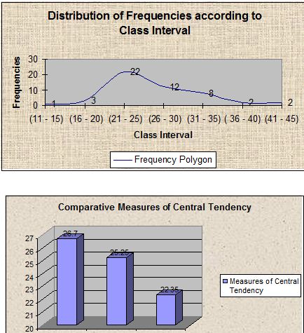
Frequency Distribution Table
Class Interval (C.I.) | Tallies | Frequency |
6 – 10 | |||| | 4 |
11 – 15 | |||| |||| |||| |||| ||| | 23 |
16 – 20 | |||| |||| || | 12 |
21 – 25 | |||| ||| | 8 |
26 – 30 | 0 | |
31 – 35 | | | 1 |
36 – 40 | || | 2 |
N = 50
4.1.1 Measures of Central Tendency
4.1.1.1 The Mean
# True Mean = A.M.+(Σfd/N)i
C.I. | Mid point | Frequency (f) | Deviation (d) | Product (fd) |
6 – 10 | 8 | 4 | – 1 | – 4 |
11 – 15 | 13 | 23 | 0 | 0 |
16 – 20 | 18 | 12 | + 1 | + 12 |
21 – 25 | 23 | 8 | + 2 | + 16 |
26 – 30 | 28 | 0 | + 3 | 0 |
31 – 35 | 33 | 1 | + 4 | + 4 |
36 – 40 | 38 | 2 | + 5 | + 10 |
N = 50 Σfd = 38
| Here – A.M.= 13; i = 5 N = 50 Σfd = 38 |
True Mean = A.M.+(Σfd/N)i
= 13 + (38/50) 5
= 13 + (0.76) 5
= 13 + 3.8
= 16.8
| Mean = 16.8 |
4.1.1.2 The Median
# Median = L+{(N/2-cfu)/fm}i
C.I. | Lower and upper limit of C.I. | Frequency (f) | Cumulative Frequency (cfu) |
6 – 10 | 5.5 – 10.5 | 4 | 4 |
11 – 15 | 10.5 – 15.5 | 23 | 27 |
16 – 20 | 15.5 – 20.5 | 12 | 39 |
21 – 25 | 20.5 – 25.5 | 8 | 47 |
26 – 30 | 25.5 – 30.5 | 0 | 47 |
31 – 35 | 30.5 – 35.5 | 1 | 48 |
36 – 40 | 35.5 – 40.5 | 2 | 50 |
| Here- L = 10.5 Cfu = 4 fm = 23 i = 5 N = 50 |
Median = L+{(N/2-cfu)/fm}i
= 10.5 +{(25 – 4)/ 23} 5
= 10.5 + (21/23) 5
= 10.5 + (0.913) 5
= 10.5 + 4.57
= 15.07 (Apprx.)
| Median = 15.07 |
4.1.1.3 The Mode
Mode = 3 median – 2 mean
= 3 x 15.07 – 2 x 16.8
= 45.21 – 33.6
= 11.61
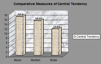
| Mode = 11.61 |
Comment
The value of mean, median and mode is respectively 16.8, 15.07 and 11.61.The value of mean and median is nearer to each other; but mode is in pretty much distance. Here 11 – 15 class interval contains maximum number of frequency, but mean and median don’t belong to that class interval.11 – 15 and 16 – 20 class intervals contain a total of 35 scores together, that is 70% of the total score. It shows that the scores have significant central tendency; but the value of mode indicates that the distribution would be positively skewed.
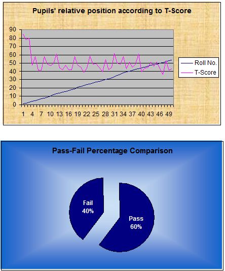
4.1.3 Measures of Relative Positions
Major measures of relative positions are percentile ranks, Z-score and T-score. I shall determine only Z-score and T-score here as they are more reliable than percentile ranks.
S.D. has been calculated as 6.5.
# Standard score (Z – Score), Z = (X – M) / s
# T = 50 + 10Z
Student’s Roll No.
| Z –score (Z = (X-M)/ s) | T-score (T = 50 + 10Z) |
01 | (39 – 16.8) / 6.5 = 3.42 | 84.5 |
02 | (35 – 16.8) / 6.5 = 2.80 | 78 |
03 | (36 – 16.8) / 6.5 = 2.95 | 79.5 |
04 | (15 – 16.8) / 6.5 = – 0.28 | 47.2 |
05 | (22 – 16.8) / 6.5 = 0.80 | 58 |
06 | (11 – 16.8) / 6.5 = – 0.89 | 41.1 |
07 | (11 – 16.8) / 6.5 = – 0.89 | 41.1 |
08 | (22 – 16.8) / 6.5 = 0.80 | 58 |
09 | (16 – 16.8) / 6.5 = – 0.12 | 48.8 |
10 | (14.5 – 16.8) / 6.5 = – 0.35 | 46.5 |
12 | (16.5 – 16.8) / 6.5 = – 0.04 | 49.6 |
13 | (24 – 16.8) / 6.5 = 1.11 | 61.1 |
14 | (13 – 16.8) / 6.5 = – 0.58 | 44.2 |
15 | (11.5 – 16.8) / 6.5 = – 0.82 | 41.8 |
16 | (15 – 16.8) / 6.5 = – 0.28 | 47.2 |
17 | (11.5 – 16.8) / 6.5 = -0.82 | 41.8 |
18 | (11.5 – 16.8) / 6.5 = – 0.82 | 41.8 |
19 | (22 – 16.8) / 6.5 = 0.80 | 58 |
21 | (15 – 16.8) / 6.5 = – 0.28 | 47.2 |
22 | (13.5 – 16.8) / 6.5 = – 0.51 | 44.9 |
23 | (9.5 – 16.8) / 6.5 = – 1.12 | 38.8 |
24 | (12.5 – 16.8) / 6.5 = – 0.66 | 43.4 |
25 | (22.5 – 16.8) / 6.5 = 0.88 | 58.8 |
26 | (16 – 16.8) / 6.5 = – 0.12 | 48.8 |
27 | (16.5 – 16.8) / 6.5 = – 0.04 | 49.6 |
28 | (13 – 16.8) / 6.5 = – 0.58 | 44.2 |
29 | (10 – 16.8) / 6.5 = -1.05 | 39.5 |
30 | (19.5 – 16.8) / 6.5 = 0.42 | 54.2 |
31 | (11.5 – 16.8) / 6.5 = – 0.82 | 41.8 |
32 | (13.5 – 16.8) / 6.5 = – 0.51 | 44.9 |
33 | (24.5 – 16.8) / 6.5 = 1.18 | 61.8 |
35 | (17 – 16.8) / 6.5 = 0.03 | 50.3 |
36 | (16 – 16.8) / 6.5 = – 0.12 | 48.8 |
38 | (22 – 16.8) / 6.5 = 0.80 | 58 |
39 | (12 – 16.8) / 6.5 = – 0.74 | 42.6 |
40 | (17.5 – 16.8) / 6.5 = 0.11 | 51.1 |
41 | (13.5 – 16.8) / 6.5 = – 0.51 | 44.9 |
42 | (16 – 16.8) / 6.5 = – 0.12 | 48.8 |
43 | (24 – 16.8) / 6.5 = 1.11 | 61.1 |
44 | (10 – 16.8) / 6.5 = – 1.05 | 39.5 |
45 | (12.5 – 16.8) / 6.5 = – 0.66 | 43.4 |
46 | (13 – 16.8) / 6.5 = – 0.58 | 44.2 |
47 | (17.5 – 16.8) / 6.5 = 0.11 | 51.1 |
48 | (14 – 16.8) / 6.5 = – 0.43 | 45.7 |
49 | (16 – 16.8) / 6.5 = 0.12 | 51.2 |
50 | (12.5 – 16.8) / 6.5 = – 0.66 | 43.4 |
51 | (8 – 16.8) / 6.5 = – 1.35 | 36.5 |
52 | (19 – 16.8) / 6.5 = 0.34 | 53.4 |
53 | (11 – 16.8) / 6.5 = – 0.89 | 41.1 |
54 | (12 – 16.8) / 6.5 = – 0.74 | 42.6 |
Comment
From this table relative position of any student in comparison to other or whole as a group can easily be made. The T-score shown above itself is a comprehensive presentation of relative position. Scores above 50 are more than average; scores below 50 are less than average.
4.1.4 Grading of Test-1 Results
Norm of Grading
Norm | Number Range (Apprx.) | Grade | GPA |
Mean + 2.5 S.D. & above | 33 and above | A | 4.00 |
Mean +1.5 S.D. – up to Mean + 2.5 S.D. | 27 -32 | B | 3.50 |
Mean + 0.5 S.D. – up to Mean + 1.5 S.D. | 20 – 26 | C | 3.00 |
Mean – 0.5 S.D.-up to Mean + 1.5 S.D. | 14 – 19 | D | 2.50 |
Below Mean | 0 – 13 | F | —— |
Grading of students
Roll No. | Obtained Mark | Grade | GPA |
01 | 39 | A | 4.00 |
02 | 35 | A | 4.00 |
03 | 36 | A | 4.00 |
04 | 15 | D | 2.50 |
05 | 22 | C | 3.00 |
06 | 11 | F | —— |
07 | 11 | F | —— |
08 | 22 | C | 3.00 |
09 | 16 | D | 2.50 |
10 | 14.5 | D | 2.50 |
12 | 16.5 | D | 2.50 |
13 | 24 | C | 3.00 |
14 | 13 | F | —— |
15 | 11.5 | F | —— |
16 | 15 | D | 2.50 |
17 | 11.5 | F | —— |
18 | 11.5 | F | —— |
19 | 22 | C | 3.00 |
21 | 15 | D | 2.50 |
22 | 13.5 | D | 2.50 |
23 | 9.5 | F | —— |
24 | 12.5 | F | —— |
25 | 22.5 | C | 3.00 |
26 | 16 | D | 2.50 |
27 | 16.5 | D | 2.50 |
28 | 13 | F | —— |
29 | 10 | F | —— |
30 | 19.5 | C | 3.00 |
31 | 11.5 | F | —— |
32 | 13 | F | —— |
33 | 24.5 | C | 3.00 |
35 | 17 | D | 2.50 |
36 | 16 | D | 2.50 |
38 | 22 | C | 3.00 |
39 | 12 | F | —— |
40 | 17.5 | D | 2.50 |
41 | 13.5 | D | 2.50 |
42 | 16 | D | 2.50 |
43 | 24 | C | 3.00 |
44 | 10 | F | —— |
45 | 12.5 | F | —— |
46 | 13 | F | —— |
47 | 17.5 | D | 2.50 |
48 | 14 | D | 2.50 |
49 | 16 | D | 2.50 |
50 | 12.5 | F | —— |
51 | 8 | F | —— |
52 | 19 | D | 2.50 |
53 | 11 | F | —— |
54 | 12 | F | —— |
It is to be noted that this grading was not executed in the school’s test result; it is done only to fulfill the purpose of statistical analysis report. Combined score of MCQ and Essay type test was executed for grading of students and that result was submitted to school. Then the score was converted into 15 and was added as class test number.
Percentage of pass and Fail
P/F | No. of students | Percentage |
Pass | 30 | 60% |
Fail | 20 | 40% |
Percentage of grading
Grade | No. of students | Percentage |
A | 3 | 6% |
B | 0 | 0% |
C | 9 | 18% |
D | 18 | 36% |
F | 20 | 40% |
4.1.5 Graphic presentation of Test-1 result analysis
4.2 Analysis of Test-2 results (MCQ test)
Student’s score in Test-2
Roll No. | Obtained Mark (Out of 50) | Roll No. | Obtained Mark (Out of 50) |
01 | 43 | 36 | 34 |
02 | 36 | 38 | 33 |
03 | 43 | 39 | 21 |
04 | 29 | 40 | 34 |
05 | 30 | 41 | 25 |
06 | 31 | 42 | 23 |
07 | 24 | 43 | 27 |
08 | 33 | 44 | 38 |
09 | 23 | 45 | 23 |
10 | 27 | 46 | 23 |
12 | 25 | 47 | 27 |
13 | 25 | 48 | 20 |
14 | 15 | 49 | 22 |
15 | 30 | 50 | 18 |
16 | 29 | 51 | 29 |
17 | 24 | 52 | 25 |
18 | 24 | 53 | 23 |
19 | 27 | 54 | 29 |
21 | 28 | N=50 | |
22 | 25 | ||
23 | 24 | ||
24 | 24 | ||
25 | 32 | ||
26 | 23 | ||
27 | 32 | ||
28 | 24 | ||
29 | 33 | ||
30 | 27 | ||
31 | 22 | ||
32 | 19 | ||
33 | 25 | ||
35 | 25 | ||
Tabulation of scores
# Number of the class = (Range/class Interval) +1
= {(Highest score-Lowest score)/Class Interval}+1
= {(43 – 15)/5}+1
= (28/5)+1
= 5.6 + 1
= 6.6
= 7 (in full number)
Frequency Distribution Table
Class Interval (C.I.) | Tallies | Frequency |
11 -15 | | | 1 |
16 – 20 | ||| | 3 |
21 – 25 | |||| |||| |||| |||| || | 22 |
26 – 30 | |||| |||| || | 12 |
31 – 35 | |||| ||| | 8 |
36 – 40 | || | 2 |
41 – 45 | || | 2 |
N = 50
4.2.1 Measures of Central Tendency
4.2.1.1 The Mean
# True Mean = A.M.+(Σfd/N)i
| C.I. | Mid point | Frequency (f) | Deviation (d) | Product (fd) |
11 -15 | 13 | 1 | -2 | – 2 |
16 – 20 | 18 | 3 | – 1 | – 3 |
21 – 25 | 23 | 22 | 0 | 0 |
26 – 30 | 28 | 12 | + 1 | + 12 |
31 – 35 | 33 | 8 | + 2 | + 16 |
36 – 40 | 38 | 2 | + 3 | + 6 |
41 – 45 | 43 | 2 | + 4 | + 8 |
N = 50 Σfd = 37
| Here – A.M.= 23 N = 50 Σfd = 37 i = 5 |
True Mean = A.M.+(Σfd/N)i
= 23 + (37/50) 5
= 23 + (0.74) 5
= 23 + 3.7
= 26.7
| Mean = 26.7 |
4.2.1.2 The Median
# Median = L+{(N/2-cfu)/fm}i
C.I. | Lower and upper limit of C.I. | Frequency (f) | Cumulative Frequency (cfu) |
11 -15 | 10.5 – 15.5 | 1 | 1 |
16 – 20 | 15.5 – 20.5 | 3 | 4 |
21 – 25 | 20.5 – 25.5 | 22 | 26 |
26 – 30 | 25.5 –30.5 | 12 | 38 |
31 – 35 | 30.5 – 35.5 | 8 | 46 |
36 – 40 | 35.5 – 40.5 | 2 | 48 |
41 – 45 | 40.5 – 45.5 | 2 | 50 |
| Here- L = 20.5 Cfu = 4 fm = 22 i = 5 N = 50 |
Median = L+{(N/2-cfu)/fm}i
= 20.5 +{(25 – 4)/ 22} 5
= 20.5 + (21/22) 5
= 20.5 + (0.95) 5
= 20.5 + 4.75
= 25.25 (Apprx.)
| Median = 25.25 |
4.2.1.3 The Mode
Mode = 3 median – 2 mean
= 3 x 25.25 – 2 x 26.7
= 75.75 – 53.4
= 22.35
Mode = 22.35 |
Comment
The value of mean, median and mode is respectively 26.7, 25.25 and 22.35.The value of mean and median is nearer to each other; but mode is in some distance. Here 21 – 25 class interval contains maximum number of frequency, but mean and median don’t belong to that class interval.21 – 25 and 26 – 30 class intervals contain a total of 34 scores together, that is 68% of the total score. It shows that the scores have significant central tendency; but the value of mode indicates that the distribution would be a little positively skewed.
4.2.3 Measures of Relative Positions
Major measures of relative positions are percentile ranks, Z-score and T-score. I shall determine only Z-score and T-score here as they are more reliable than percentile ranks.
# Standard score (Z – Score), Z = (X – M) / s
# T = 50 + 10Z
Student’s Roll No.
| Z –score (Z = (X-M)/ s) | T-score (T = 50 + 10Z) |
01 | (43 – 26.7) / 6.05 = 2.69 | 76.9 |
02 | (36 – 26.7) / 6.05 = 1.54 | 65.4 |
03 | (43 – 26.7) / 6.05 = 2.69 | 76.9 |
04 | (29 – 26.7) / 6.05 = 0.38 | 53.8 |
05 | (30 – 26.7) / 6.05 = 0.54 | 55.4 |
06 | (31 – 26.7) / 6.05 = 0.71 | 57.1 |
07 | (24 – 26.7) / 6.05 = – 0.45 | 45.5 |
08 | (33 – 26.7) / 6.05 = 1.04 | 60.4 |
09 | (23 – 26.7) / 6.05 = – 0.61 | 43.9 |
10 | (27 – 26.7) / 6.05 = 0.05 | 50.5 |
12 | (25 – 26.7) / 6.05 = – 0.28 | 47.2 |
13 | (25 – 26.7) / 6.05 = – 0.28 | 47.2 |
14 | (15 – 26.7) / 6.05 = – 1.93 | 30.7 |
15 | (30 – 26.7) / 6.05 = 0.54 | 55.4 |
16 | (29 – 26.7) / 6.05 = 0.38 | 53.8 |
17 | (24 – 26.7) / 6.05 = – 0.45 | 45.5 |
18 | (24 – 26.7) / 6.05 = – 0.45 | 45.5 |
19 | (27 – 26.7) / 6.05 = 0.05 | 50.5 |
21 | (28 – 26.7) / 6.05 = 0.21 | 52.1 |
22 | (25 – 26.7) / 6.05 = – 0.28 | 52.8 |
23 | (24 – 26.7) / 6.05 = – 0.45 | 45.5 |
24 | (24 – 26.7) / 6.05 = – 0.45 | 45.5 |
25 | (32 – 26.7) / 6.05 = 0.88 | 58.8 |
26 | (23 – 26.7) / 6.05 = – 0.61 | 43.9 |
27 | (32 – 26.7) / 6.05 = 0.88 | 58.8 |
28 | (24 – 26.7) / 6.05 = – 0.45 | 45.5 |
29 | (33 – 26.7) / 6.05 = 1.04 | 60.4 |
30 | (27 – 26.7) / 6.05 = 0.05 | 50.5 |
31 | (22 – 26.7) / 6.05 = – 0.78 | 42.2 |
32 | (19 – 26.7) / 6.05 = – 1.27 | 37.3 |
33 | (25 – 26.7) / 6.05 = – 0.28 | 47.2 |
35 | (25 – 26.7) / 6.05 = – 0.28 | 47.2 |
36 | (34 – 26.7) / 6.05 = 1.20 | 62 |
38 | (33 – 26.7) / 6.05 = 1.04 | 60.4 |
39 | (21 – 26.7) / 6.05 = – 0.94 | 40.6 |
40 | (34 – 26.7) / 6.05 = 1.20 | 61.2 |
41 | (25 – 26.7) / 6.05 = – 0.28 | 47.8 |
42 | (23 – 26.7) / 6.05 = – 0.61 | 43.9 |
43 | (27 – 26.7) / 6.05 = 0.05 | 50.5 |
44 | (38 – 26.7) / 6.05 = 1.87 | 68.7 |
45 | (23 – 26.7) / 6.05 = – 0.61 | 43.9 |
46 | (23 – 26.7) / 6.05 = – 0.61 | 43.9 |
47 | (27 – 26.7) / 6.05 = 0.05 | 50.5 |
48 | (20 – 26.7) / 6.05 = – 1.10 | 39.9 |
49 | (22 – 26.7) / 6.05 = – 0.78 | 42.2 |
50 | (18 – 26.7) / 6.05 = – 1.43 | 35.7 |
51 | (29 – 26.7) / 6.05 = 0.38 | 53.8 |
52 | (25 – 26.7) / 6.05 = – 0.28 | 47.2 |
53 | (23 – 26.7) / 6.05 = – 0.61 | 43.9 |
54 | (29 – 26.7) / 6.05 = 0.38 | 53.8 |
Comment
From this table relative position of any student in comparison to other or whole as a group can easily be made. The T-score shown above itself is a comprehensive presentation of relative position. Scores above 50 are more than average, scores below 50 are less than average.
4.2.4 Grading of Test-2 Results
Grading of students
Roll No. | Obtained Mark | Grade | GPA |
01 | 43 | A | 4.00 |
02 | 36 | B | 3.50 |
03 | 43 | A | 4.00 |
04 | 29 | C | 3.00 |
05 | 30 | C | 3.00 |
06 | 31 | C | 3.00 |
07 | 24 | D | 2.50 |
08 | 33 | B | 3.50 |
09 | 23 | D | 2.50 |
10 | 27 | C | 3.00 |
12 | 25 | D | 2.50 |
13 | 25 | D | 2.50 |
14 | 15 | F | —— |
15 | 30 | C | 3.00 |
16 | 29 | C | 3.00 |
17 | 24 | D | 2.50 |
18 | 24 | D | 2.50 |
19 | 27 | C | 3.00 |
21 | 28 | C | 3.00 |
22 | 25 | D | 2.50 |
23 | 24 | D | 2.50 |
24 | 24 | D | 2.50 |
25 | 32 | C | 3.00 |
26 | 23 | D | 2.50 |
27 | 32 | C | 3.00 |
28 | 24 | D | 2.50 |
29 | 33 | B | 3.50 |
30 | 27 | C | 3.00 |
31 | 22 | D | 2.50 |
32 | 19 | F | —— |
33 | 25 | D | 2.50 |
35 | 25 | D | 2.50 |
36 | 34 | B | 3.50 |
38 | 33 | B | 3.50 |
39 | 21 | D | 2.50 |
40 | 34 | B | 3.50 |
41 | 25 | D | 2.50 |
42 | 23 | D | 2.50 |
43 | 27 | C | 3.00 |
44 | 38 | B | 3.50 |
45 | 23 | D | 2.50 |
46 | 23 | D | 2.50 |
47 | 27 | C | 3.00 |
48 | 20 | F | —— |
49 | 22 | D | 2.50 |
50 | 18 | F | —— |
51 | 29 | C | 3.00 |
52 | 25 | D | 2.50 |
53 | 23 | D | 2.50 |
54 | 29 | C | 3.00 |
It is to be noted that this grading was not executed in the school’s test result; it is done only to fulfill the purpose of statistical analysis report. Combined score of MCQ and Essay type test was executed for grading of students and that result was submitted to school. Then the score was converted into 15 and was added as class test number.
Percentage of pass and Fail
P/F | No. of students | Percentage |
Pass | 46 | 92% |
Fail | 4 | 8% |
Percentage of grading
Grade | No. of students | Percentage |
A | 2 | 4% |
B | 7 | 14% |
C | 15 | 30% |
D | 22 | 44% |
F | 4 | 8% |
4.2.5 Graphic Presentation of Test-2 result analysis
4.3 Correlation between Test-1 & Test-2 results
N S XY – SX SY
The Pearson, ¡ =
Ö [{NSX2 – (SX )2 }{ NSY2 – ( SY )2 }
Roll No. | Score of Test – 1 (X) | X2 | Score of Test – 2 (Y) | Y2 | XY |
1 | 39 | 1521 | 43 | 1849 | 1677 |
2 | 35 | 1225 | 36 | 1296 | 1260 |
3 | 36 | 1296 | 43 | 1849 | 1548 |
4 | 15 | 225 | 29 | 841 | 435 |
5 | 22 | 484 | 30 | 900 | 660 |
6 | 11 | 121 | 31 | 961 | 341 |
7 | 11 | 121 | 24 | 576 | 264 |
8 | 22 | 484 | 33 | 1089 | 726 |
9 | 16 | 256 | 23 | 529 | 368 |
10 | 14.5 | 210.25 | 27 | 729 | 391.5 |
12 | 16.5 | 272.25 | 25 | 625 | 412.5 |
13 | 24 | 576 | 25 | 625 | 600 |
14 | 13 | 169 | 15 | 225 | 195 |
15 | 11.5 | 132.25 | 30 | 900 | 345 |
16 | 15 | 225 | 29 | 841 | 435 |
17 | 11.5 | 132.25 | 24 | 576 | 276 |
18 | 11.5 | 132.25 | 24 | 576 | 276 |
19 | 22 | 484 | 27 | 729 | 594 |
21 | 15 | 225 | 28 | 784 | 420 |
22 | 13.5 | 182.25 | 25 | 625 | 337.5 |
23 | 9.5 | 90.25 | 24 | 576 | 228 |
24 | 12.5 | 156.25 | 24 | 576 | 300 |
25 | 22.5 | 506.25 | 32 | 1024 | 720 |
26 | 16 | 256 | 23 | 529 | 368 |
27 | 16.5 | 272.25 | 32 | 1024 | 528 |
28 | 13 | 169 | 24 | 576 | 312 |
29 | 10 | 100 | 33 | 1089 | 330 |
30 | 19.5 | 380.25 | 27 | 729 | 526.5 |
31 | 11.5 | 132.25 | 22 | 484 | 253 |
32 | 13 | 169 | 19 | 361 | 247 |
33 | 24.5 | 600.25 | 25 | 625 | 612.5 |
35 | 17 | 289 | 25 | 625 | 425 |
36 | 16 | 256 | 34 | 1156 | 544 |
38 | 22 | 484 | 33 | 1089 | 726 |
39 | 12 | 144 | 21 | 441 | 252 |
40 | 17.5 | 306.25 | 34 | 1156 | 595 |
41 | 13.5 | 182.25 | 25 | 625 | 337.5 |
42 | 16 | 256 | 23 | 529 | 368 |
43 | 24 | 576 | 27 | 729 | 648 |
44 | 10 | 100 | 38 | 1444 | 380 |
45 | 12.5 | 156.25 | 23 | 529 | 287.5 |
46 | 13 | 169 | 23 | 529 | 299 |
47 | 17.5 | 306.25 | 27 | 729 | 472.5 |
48 | 14 | 196 | 20 | 400 | 280 |
49 | 16 | 256 | 22 | 484 | 352 |
50 | 12.5 | 156.25 | 18 | 324 | 225 |
51 | 8 | 64 | 29 | 841 | 232 |
52 | 19 | 361 | 25 | 625 | 475 |
53 | 11 | 121 | 23 | 529 | 253 |
54 | 12 | 144 | 29 | 841 | 348 |
N = 50 | ∑X = 827 | ∑X2 = 15828.5 | ∑Y = 1355 | ∑Y2 = 38343 | ∑XY = 23486 |
Comment
The value of correlation between Test-1 & Test-2 is +0.58. That indicates the tests have a positive, substantial and marked relationship. The two tests scores have a tendency to vary in the same direction. For example: a student who has done well in test-1 has a high chance to do well in Test-2 and a student who could not do well in Test-1 has a high chance to score low in Test-2 and vise versa. This relationship is substantial and marked.
4.4 Graphic comparison between Test-1 & Test-2 results
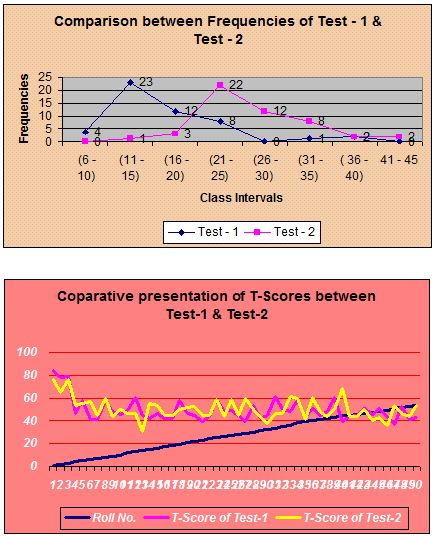
Comment
Frequency distributions are not similar. Values of mean, median and mode of Test-2 are much higher than that of mean, median and mode of Test-1. That indicates students have done much well in MCQ exam than essay type exam. Pass rate was also improved in Test –2. Pass rate of Test-2 is 92% while it was 60% in Test-1. Comparatively better grades (A, B, C) was achieved in higher frequency in Test-2 than Test-1. MCQ score distribution is comparatively normal than that of essay type score distribution. Students’ T-Score is comparatively better in Test-2.
5.0 Analysis of combined Test and Test scores ( Essay type + MCQ together )
I felt it is necessary to make an analysis of combined test and test scores of essay type and MCQ by summing up their scores in order to get an overall idea about the test and test results. Moreover a student, who has scored in essay type, may score well in MCQ type and vise versa. So there is a high chance of getting a new set of central tendencies, variabilites and relative positions. It is also noted earlier that the score of MCQ and essay type separately was not used for grading. A sum up score of essay type and MCQ scores was used for grading. Student’s score out of 100 was graded and submitted to school by converting into 15 as the result of class test.
6.0 Ending Remarks
I believe that the students of class seven (B) have the ability to do well. I have got them very intelligent, curious and participating in the class. They have interests in pleasant studies. Before joining the school since leaving and till now I have heard it many times that the quality of the students of Engineering University Higher Secondary School is average. But as I have experienced them to my experiences and score shows that they are excellent.