The central limit theorem (CLT) in probability theory is a statistical principle that states that if the sample size is large enough, the sample means distribution of a random variable will assume a near-normal or normal distribution. The hypothesis is a critical idea in the likelihood hypothesis since it infers that probabilistic and measurable techniques that work for typical disseminations can be appropriate to numerous issues including different kinds of dispersions. In other words, CLT is a statistical theory that, provided that a population with a finite level of variance has a sufficiently large sample size, the mean of all samples from the same population will be approximately equal to the mean of the population. In addition, all the samples will follow an approximate normal pattern of distribution, with all variances being roughly equal to the population variance, divided by the size of each sample.
The ideal helpful estimation is given by as far as a possible hypothesis, which in the exceptional instance of the binomial dispersion was first found by Abraham de Moivre around 1730; it wasn’t officially named until 1930, when noted Hungarian mathematician George Polya authoritatively named it the Central Limit Theorem. Let X1,…, Xn be random independent variables that have a common distribution with μ expectation and σ2 variance. There are several variations to the central limit theorem. Random variables must be distributed identically in their common form. In variations, for non-identical distributions or for non-independent measurements, the convergence of the mean to the normal distribution often occurs if certain conditions are met. The earliest version of this theorem, the de Moivre-Laplace theorem, is that the normal distribution can be used as an approximation to the binomial distribution.
Quite possibly the main part of the hypothesis is that the mean of the example will be the mean of the whole populace. On the off chance that we ascertain the mean of different examples of the populace, add them up, and locate their normal, the outcome will be the gauge of the populace mean.
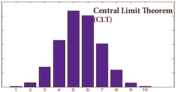
When using standard deviation, the same applies. The result will be the standard deviation of the whole population if we calculate the standard deviation of all the samples in the population, add them up, and find the average. The law of large numbers implies that the distribution of the random variable X̄n = n−1(X1 +⋯+ Xn) is essentially just the degenerate distribution of the constant μ, because E(X̄n) = μ and Var(X̄n) = σ2/n → 0 as n → ∞. The standardized random variable (X̄n − μ)/(σ/√n) has mean 0 and variance 1. As a general rule, sample sizes equal to or greater than 30 are considered adequate to hold the CLT, which implies that the distribution of the means of the sample is usually equally distributed. Therefore, the more samples one takes, the more the results that are graphed take the form of regular distribution.
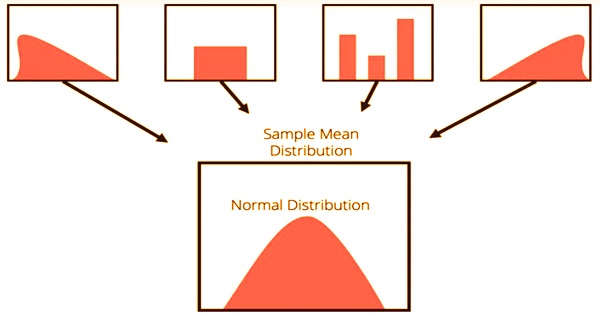
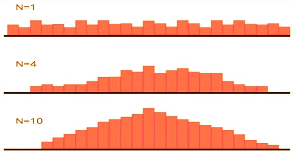
The central limit theorem forms the foundation of the distribution of probability. When subject to repeated sampling, it makes it easy to understand how population estimates behave. The theorem shows the shape of the distribution formed by the means of repeated population samples when plotted on a graph. Additionally, the populace is generally delineated into moderately homogeneous gatherings, and the review is intended to exploit this separation. As the example sizes get greater, the dissemination of the methods from the rehashed tests will in general standardize and take after a typical dispersion. The outcome remains the same regardless of what the distribution’s initial form was. This can be seen in the figure below:
Due to the relative ease of producing the required financial data, the CLT is useful when analyzing the returns of an individual stock or wider indices, since the analysis is simple. As a result, investors of all kinds rely on the CLT to evaluate stock yields, construct portfolios, and manage risk. Valuable speculation of a grouping of autonomous, indistinguishably appropriated arbitrary factors is a blending irregular cycle in discrete time; “blending” signifies, generally, that arbitrary factors transiently far separated from each other are almost free. A few sorts of blending are utilized in the ergodic hypothesis and likelihood hypothesis.
Pierre-Simon Laplace, another prominent French mathematician, reintroduced the term (CLT) in 1812. In his work titled “Théorie Analytique des Probabilités”, Laplace re-introduced the normal distribution principle in an effort to approximate binomial distribution with the normal distribution. The mathematician found that the normal of free irregular factors, when expanded in number, will, in general, follow ordinary dissemination. Around then, Laplace’s discoveries on as far as possible hypothesis stood out from different scholars and academicians.
There has been much effort to generalize both the rule of large numbers and the central limit theorem so that it is unnecessary for the variables to be either independent or distributed identically. Later, in 1901, Aleksandr Lyapunov, a Russian mathematician, extended the central limit theorem. Lyapunov proceeded to characterize the idea all in all terms and demonstrate how the idea functioned numerically. The trademark capacities that he used to give the hypothesis were received in the current likelihood hypothesis. In order to differentiate it from the “strong law,” a conceptually different outcome discussed below in the section on infinite probability spaces, the law of large numbers discussed above is also called the “weak law of large numbers.”
Only an asymptotic distribution is given by the central limit theorem. It provides a rational approximation only when close to the height of the normal distribution as an approximation for a finite number of observations; it takes a very large number of observations to extend into the tails. In particular, the CLT refers to sums of discrete random variables which are independent and identically distributed.
Information Sources: