All praise goes to almighty Allah, without His endless mercy I could not reach so close to my destination, for the time being. Simultaneously I am remembering my prophet Hazrat Mohammad (SM), the supreme guide to knowledge and wisdom for mankind.
I have the pleasure to express my deepest gratitude and indebtedness to my reverend supervisor, Dr. Mahbub Kabir, professor, Department of chemistry, Jahangirnagar University, Savar, Dhaka, for his indispensable guidance, encouragement and suggestions throughout the period of my research.
I am particularly grateful to our honorable teacher Prof. Dr. Ilias Mollah, Chairman, Department of chemistry, Jahangirnagar University, Savar, Dhaka, for his kind co-operation fruitful discussions and spontaneous help out.
I am also grateful and indebted to Dr. Menarul Islam, Assistant Professor, Department of chemistry, Jahangirnagar University, Savar, Dhaka, for his indispensable guidance, encouragement and suggestions throughout the period of my research.
I also take this opportunity to express my gratefulness to all of my honorable teachers of the Department of chemistry, Jahangirnagar University, for their help and co-operation.
I would like to pay my respect and gratefulness to Md. Abdul Kuddus and Subir chowdhury, PhD researcher in physical laboratory for their utmost help to me during my thesis work.
I offer my grateful to Md. Mohibullah Khan Sowrav, Md. Rasedul Islam Ripon and Abul Kalam Azad for their utmost help to me during my thesis work.
I want to give thanks to all of my friends for their co-operation and help during the course of my lab work.
I offer my heartfelt thanks to my brothers for their constant inspiration. Finally I express my deepest gratitude and sincere thanks to my parents for keeping me in their good wishes forever.
2.1 REAGENTS AND CHEMICALS
A list of the chemicals is given below:
- Ferrous Sulphate (Ana. R.) : B. D. H. England
- Copper Sulphate (Ana. R.) : Ridel –dettean
- Cadmium Sulphate (Ana. R.) : B. D. H. England
- Potassium chloride (R.) : B. D. H. England
- Dioxane ( R.) : Ridel –dettean
Iron, cadmium and copper sulphates of analytical reagent grade were recrystallized twice from conductivity water at a temperature between 10 and 20 and then dried at room temperature. Reagent grade 1,4-dioxane was fractionally distilled after being dried to remove traces of water. Potassium chloride used for the cell calibration was reagent grade and was recrystallized three times from conductivity water. It was then dried in vacuum at 200 for more than one week.
Dioxane-water mixtures were carefully prepared by using conductivity water (specific conductivity < 2 10-6 Scm-1 at 25 ). Solutions of different concentrations were carefully prepared by using dioxane – water mixture.
2.2 CONDUCTIVITY WATER
Water used in conductance was deionized water purified by passing it through a double Barnsted ion- exchange column (organic materials exchange and mixed cation – anion exchange). The conductance of this water was monitored by measuring the conductance during the collection. The value was < 1 10-6 Scm2 at room temperature.
2.3 MEASUREMENT OF DENSITY, VISCOSITY AND DIELECTRIC CONSTANT
The density of pure liquid and mixtures of liquids were measured by weighing a definite volume of the liquid in a density bottle. The viscosity of dioxane – water mixtures were measured experimentally by using Oswald viscometer. The dielectric constant of the solvent mixtures was interpolated from the published data.36 The viscosity and dielectric constants of dioxane – water mixtures are summarized in table 1.
2.3.1 MEASUREMENT OF DENSITY
The relative density is the ratio of the weight of a given volume of the substance to the weight of an equal volume of water at the same temperature and the density of the substance at temperature T is equal to the relative density multiplied by the density of water at that temperature. Densities of liquids were measured by weighing a definite volume of the liquid in a density bottle. The densities of liquids and different solutions were calculated by the equation.
dT = DT
where
w´ = the weight of liquid or solution, w = the weight of water and
= the density of water at T
2.3.2 MEASUREMENT OF VISCOSITY
According to the poiseuelle’s equation the ratio of the viscosity coefficients of the two liquid is given by
Where, t1 and t2 are time of outflow of water and liquid respectively.
Since the pressure p1 and p2 are proportional to the densities of the two liquids d1 and d2 then
= Consequently, once d1, d2 and and are known, determination of t1 and t2 permits the calculation of , the viscosity coefficient of the liquid under consideration.
2.4 PREPARATION OF METAL SULPHATES SOLUTIONS
Solution of metal salts were prepared measuring required amount of the compound in an analytical balance and dissolving the solvent to give the appropriate value at 25 . Then solutions of different concentrations were carefully prepared by dilution of the stock solutions of metal sulphates at 25 , with increasing temperature, concentrations were changed. Solutions of different concentrations at different temperature were calculated by the equation
Where and are the concentrations of solution at temperature 25 and T respectively. d1 and d2 are the densities of solution at temperature 25 and T respectively.
2.5 CONDUCTIVITY MEASUREMENTS
The electrical conductivity of the solutions was measured at 50/60 Hz by the conductance linear – bridge method. A conductivity cell which is designated for solutions of low conductivity was used throughout this study. The conductivity cell was calibrated using 0.1 and 0.01 decimal solutions of purified fused potassium chloride. The cell constant was determined to be 0.610 cm-1 using a standard potassium chloride solution and exhibited no tendency to change with the two standard solutions. The solution in cell was magnetically stirred at a rate of 1.2 revolutions per second. The experimental error of the conductivity measurement was less than 1%. All the measurements were carried out in an electrically grounded thermostat bath containing distilled water. Temperature was controlled and measured with sensitively of 0.05 .
2.6 TABLES FOR THE PHYSICAL PROPERTIES OF DIOXANE – WATER MIXTURESAND EQUIVALENT CONDUCTIVITY OF DIFFERENT SOLUTIONS
The physical properties of dioxane – water mixtures are summarized in Table 1 and the equivalent conductance at different concentrations of ferrous sulphate, copper sulphate and cadmium sulphate solutions at different temperatures are listed in Table 2.1 to 2.12.
Table – 1: Physical properties of dioxane – water mixture.
5% Dioxane 10% Dioxane 15% Dioxane 20% Dioxane
| T | D | η mNsm-2 | D | ηmNsm-2 | D | ηmNsm-2 | D | ηmNsm-2 |
| 25 | 74.38 | 0.9664 | 69.85 | 1.0722 | 65.33 | 1.1780 | 60.80 | 1.2720 |
| 30 | 72.65 | 0.8694 | 68.20 | 0.9511 | 63.75 | 1.0451 | 59.30 | 1.1300 |
| 35 | 70.68 | 0.7826 | 66.35 | 0.8532 | 62.03 | 0.9281 | 57.70 | 1.0110 |
| 40 | 69.05 | 0.7038 | 64.80 | 0.7705 | 60.55 | 0.8381 | 56.30 | 0.9110 |
Table-2.1: Equivalent conductance (Λ) of FeSO4 in 5% (w/w) dioxane – water mixture at different temperature.
| Concentrationmol dm | ΛScm2 equ-1 | ΛScm2 equ-1 | ΛScm2 equ-1 | ΛScm2 equ-1 |
250C | 30 | 35 | 40 | |
| 2.00 10-4 | 116.50 | 130.18 | 140.32 | 151.54 |
| 4.00 10-4 | 109.08 | 124.73 | 134.25 | 144.75 |
| 6.00 10-4 | 105.25 | 117.10 | 126.05 | 138.10 |
| 8.00 10-4 | 100.10 | 112.25 | 122.20 | 133.08 |
| 12.00 10-4 | 96.05 | 108.00 | 117.00 | 128.25 |
Table-2.2: Equivalent conductance (Λ) of FeSO4 in 10% (w/w) dioxane – water mixture at different temperature.
| Concentrationmol dm-3 | ΛScm2 equ-1 | ΛScm2 equ-1 | ΛScm2 equ-1 | ΛScm2 equ-1 |
25 | 30 | 35 | 40 | |
| 2.00 10-4 | 104.50 | 118.05 | 127.25 | 138.25 |
| 4.00 10-4 | 98.05 | 111.70 | 120.50 | 130.75 |
| 6.00 10-4 | 93.29 | 104.85 | 112.50 | 121.60 |
| 8.00 10-4 | 90.00 | 100.19 | 107.00 | 115.30 |
| 12.00 10-4 | 84.50 | 94.00 | 98.00 | 106.10 |
Table -2.3: Equivalent conductance ( Λ ) of FeSO4 in 15% (w/w) dioxane – water mixture at different temperature.
| Concentrationmol dm-3 | ΛScm2 equ-1 | ΛScm2 equ-1 | ΛScm2 equ-1 | ΛScm2 equ-1 |
25 | 30 | 35 | 40 | |
| 2.00 10-4 | 91.51 | 101.08 | 110.85 | 124.05 |
| 4.00 10-4 | 84.10 | 92.73 | 102.15 | 113.60 |
| 6.00 10-4 | 79.24 | 87.30 | 96.10 | 107.08 |
| 8.00 10-4 | 75.09 | 83.00 | 91.23 | 101.75 |
| 12.00 10-4 | 71.25 | 79.15 | 87.40 | 96.10 |
Table -2.4: Equivalent conductance (Λ) of FeSO4 in 20% (w/w) dioxane – water mixture at different temperature.
| Concentration |
mol dm-3 Λ
Scm2 equ-1 Λ
Scm2 equ-1 Λ
Scm2 equ-1 Λ
Scm2 equ-1
25
30
35
40
2.00 10-4
80.15
90.25
100.23
110.75
4.00 10-4
72.52
81.54
90.75
99.50
6.00 10-4
66.50
75.50
84.10
92.00
8.00 10-4
63.75
73.25
81.50
89.10
12.00 10-4
61.24
70.50
78.00
86.05
Table –2.5: Equivalent conductance (Λ) of CuSO4 in 5% (w/w) dioxane – water mixture at different temperature.
| Concentration |
mol dm-3
Λ
Scm2 equ-1 Λ
Scm2 equ-1 Λ
Scm2 equ-1 Λ
Scm2 equ-1 25 30 35 402.00 10-4 113.95127.98141.87155.99
4.00 10-4
107.20
124.18
137.21
151.15
6.00 10-4
103.53
118.01
131.05
142.35
8.00 10-4
101.75
113.10
125.75
137.05
12.00 10-4
98.50
109.50
122.08
131.92
Table-2.6: Equivalent conductance (Λ) of CuSO4 in 10% (w/w) dioxane – water mixture at different temperature.
| Concentration |
mol dm-3
Λ
Scm2 equ-1 Λ
Scm2 equ-1 Λ
Scm2 equ-1 Λ
Scm2 equ-1 25 30 35 402.00 10-4
101.95
113.98
126.10
138.10
4.00 10-4
96.50
109.90
120.08
132.85
6.00 10-4
91.25
105.05
114.60
124.98
8.00 10-4
88.30
101.00
109.80
118.10
12.00 10-4
84.50
96.00
103.00
112.90
water mixture at different temperature.
| Concentration |
mol dm-3
Λ
Scm2 equ-1 Λ
Scm2 equ-1 Λ
Scm2 equ-1 Λ
Scm2 equ-1
25
30
35
40
2.00 10-4
89.96
99.98
112.15
122.75
4.00 10-4
83.50
95.87
107.00
116.98
6.00 10-4
78.25
90.00
98.75
108.25
8.00 10-4
74.10
83.15
93.10
102.85
12.00 10-4
70.30
78.50
87.00
95.00
Table-2.8: Equivalent conductance (Λ) of CuSO4 in 20% (w/w) dioxane – water mixture at different temperature.
| Concentration |
mol dm-3 Λ
Scm2 equ-1 Λ
Scm2 equ-1 Λ
Scm2 equ-1 Λ
Scm2 equ-1
25
30
35
40
2.00 10-4
79.15
88.10
99.50
107.90
4.00 10-4
71.25
82.90
93.00
102.10
6.00 10-4
67.20
74.70
83.25
93.30
8.00 10-4
64.10
67.12
78.50
85.50
12.00 10-4
59.00
62.80
72.00
77.10
Table-2.9: Equivalent conductance (Λ) of CdSO4 in 5% (w/w) dioxane – water mixture at different temperature.
| Concentration |
mol dm-3
Λ
Scm2 equ-1 Λ
Scm2 equ-1 Λ
Scm2 equ-1 Λ
Scm2 equ-1
25
30
35
40
2.00 10-4
118.25
131.70
141.00
152.50
4.00 10-4
110.50
125.50
135.25
145.75
6.00 10-4
106.00
119.20
127.00
139.25
8.00 10-4
102.06
113.00
122.20
134.50
12.00 10-4
97.15
109.00
118.00
129.30
Table-2.10: Equivalent conductance (Λ) of CdSO4 in 10% (w/w) dioxane –water mixture at different temperature.
| Concentration |
mol dm-3
Λ
Scm2 equ-1 Λ
Scm2 equ-1 Λ
Scm2 equ-1 Λ
Scm2 equ-1
25
30
35
40
2.00 10-4
106.50
119.75
128.00
139.25
4.00 10-4
99..00
112.50
121.20
132.10
6.00 10-4
94.10
106.25
116.50
126.00
8.00 10-4
91.00
101.30
110.15
120.20
12.00 10-4
86.30
96.00
106.00
116.50
Table-2.11: Equivalent conductance (Λ) of CdSO4 in 15% (w/w) dioxane – water mixture at different temperature.
| Concentration |
mol dm-3
Λ
Scm2 equ-1 Λ
Scm2 equ-1 Λ
Scm2 equ-1 Λ
Scm2 equ-1
25
30
35
40
2.00 10-4
93.50
103.00
111.50
124.75
4.00 10-4
86.00
94.75
103.10
115.60
6.00 10-4
81.20
89.30
97.30
109.00
8.00 10-4
77.00
85.00
92.00
103.75
12.00 10-4
73.25
82.15
88.40
98.00
Table-2.12: Equivalent conductance (Λ) of CdSO4 in 20% (w/w) dioxane – water mixture at different temperature.
| Concentration |
mol dm-3
Λ
Scm2 equ-1 Λ
Scm2 equ-1 Λ
Scm2 equ-1 Λ
Scm2 equ-1
25
30
35
40
2.00 10-4
82.10
92.25
102.30
112.75
4.00 10-4
74.50
83.50
92.75
101.50
6.00 10-4
68.50
77.50
85.10
93.70
8.00 10-4
65.15
74.25
82.50
90.15
12.00 10-4
60.25
71.50
79.00
87.05
3.1 DATA TREATMENT
For the treatment of the data the Fuoss-Onsagar equation in the form for an associated symmetrical electrolyte was used .
Λ = Λ0 – S(cγ) 1/2 + Ecγ log(cγ) + Jcγ – KA (cγ) f±2 Λ (3.1)
Where Λ0 is the limiting equivalent conductivity, c is the molar concentration, γ is the degree of dissociation, S is the Onsager limiting slope, E and J are theoretical coefficients, and f± is the mean ionic activity coefficient.
For the actual analysis of the association, the Fuoss“ y – x ” method was used.
Introducing some new variables defined by Fuoss by the equation:
Λ׳ = Λ + S (cγ)1/2 – Ecγ log (cγ) (3.2)
Δ Λ = Λ׳ – Λ0 (3.3)
y = Δ Λ / c γ (3.4)
and x = f±2 Λ (3.5)
The equation (3.1) is transformed into a simple form
y = J – KA x (3.6)
Equation (3.6) implies that if the variables x and y are known, the values of J and KA can be determined by a plot of y against x ( the y–x plot).The coefficient, J is a function of ion size parameter and is used for the evaluation of ‘a’ the closest distance of approach between the oppositely charged ions .
In order to compute y, values of γ and Λ0 are needed. The terms in E and J are of opposite sign, if they are both neglected the conductance equation reduces to
Λ = γ (Λ0 – Sc1/2 γ 1/2)
This is the modified form of the Oswald dilution law used formerly for analysis of conductance data.37,38
The starting approximation for γ is obtained by the classical Onsager equation :
= Λ / [Λ0 – S (c. Λ / Λ0 )1/2] (3.7)
Λ0 is estimated from the intercept on y axis of the plot of Λ vs √c. S is Onsager limiting slope of the above plot and the observed ‘S’ value is used . Λ0 is used to compute E, Λ, Λ’ and x.
For the initial calculation of x, the mean activity coefficient f±2 is estimated by the following equation.39
–log f±2 = (3.8)
Here Ka .2 for dilute solution.40
Trial values of Λ0 are used in ΔΛ and y until correct one is found, the “correct”40 one is taken as the value which linearize the ‘y-x’ plot. Too small trial value gives a curve which is concord upwards, while too large a Λ0 value leads to a ‘y-x’ plots which is concave downwards. From the ‘y-x’ plot we get Λ0,KA, a through J.
A series of calculations are done for a set of Λ0 values using equation (3.7) and (3.2) to calculate a fitting parameter for the y-x line for each Λ0 originally using 1 or 2 Λ0 unit until increments. Then Λ0 is selected which gives the best fit and the whole calculation is repeated with smaller increment of Λ0 This process is continued until the increment are only 0.01 Λ0 units. Then for higher approximation, γi ( i= 2 , 3 . . . ) is calculated by the equation
γi = Λ/ ( Λ0 – S ( cγi-1 )1/2 + Ecγi-1 log cγi-1 + J cγi-1) ( 3.9 )
where, on the right hand side, the first approximation for γ from (3.7) and the values just obtained for Λ0 and J are used. The calculation is repeated using equation (3.9) until γ (in) = γ (out) i.e., γn-1 = γn. This values of γ is used to calculated Λ’ i. e., Λ0 from equation (3.2). For any small difference in Λ0 values between the two, a second time Λ0 fixation is carried out using equation (3.9) and (3.2).
For the calculation of x at second time, the mean activity coefficient, f± is estimated by means of the Debye-Huckel equation.
–log f±2 = – (3.10)
where z (z = |z+| = |z–| for a symmetrical electrolyte) is charge number; I,the ionic strength, and A and B, the theoretical coefficients.
where
A =
and B =
In the calculation of f± by above equation, the initial ‘a’ is obtained from the initial J is used.
Then a final “y-x” plot is made. From this we get final Λ0,KA and aJ through J.
Calculation of aJ from J
In the equation for J from the relation J = Ϭ1 Λ0 + Ϭ2, different trial values of ‘a’ is used. The values of ‘a’ which fits the J equation is desired aJ value. The equation (3.1) is a three- parameter equation in Λ0, the equivalent at infinite dilution; J the coefficient of the linear term, and KA, the association constant. The symbols in equation (3.1) are the same as used by Fuoss in his monograph38,41 adopted properly to 2:2 electrolytes by the introduction of valences z.
The various coefficients then read for homologues electrolytes
where | z+ | = | z–| = | z | = z.
S = α Λ0 + β = z3 Λ0 + z2
E = E1 Λ0 – E2 = z6 Λ0 –
J = Ϭ1 Λ0 + Ϭ2
= {1012 z6 [ h(b) + 0.9074 + ln ( )]} Λ0 +
z5 + z3a
– z2 (1.0170 + ln )
Where
h(b) = (2b2 +2b – 1) / b3
b =
K =
–log f±2 =
The calculation of the various coefficients is shown below:
We know
k = √ (
where k is the gas constant per molecule i.e., R / N , T the absolute temperature, and ni the number of any given kind of ions per cubic centimeter of solution.
The concentration of ions c in gram ionic weight per liter from the density .
c = 1000
Then
k = √ ( )
Here, z+ = z – = z for homologues electrolytes.
= √ ( )
= √ ( ) z √ c
Here, e = electronic charge = 4.80298 10-10e.s.u.
K = Boltzmann constant
= 1.38054 10-16 erg.deg-1
k = √ ( z √ C
or, k = z √ c
b = = z2
= z2
E1 = 2.3026 (k2 a2 b2 / 24 c) =
E2 = 2.3026 (k a b β / 16 c 1/2)
= 2.3026
ð E2 =
Ϭ1 = ( k2 a2 b2 /12 c ) [ h ( b ) + 0.9074 + ln ( )
= Z6 [ h ( b ) + 0.9074 + ln ( ) ]
Ϭ2 = α β + (11 β Ka / 12 c 1/2) – (ka b β / 8 c 1/2) [1.0170 + ln ( )]
= z5 + z3a
– z2 (1.0170 + ln )
Calculation of Ϭ1 and Ϭ2
Ϭ1 and Ϭ2 for dioxane – water mixtures at different temperatures.
For 5 % (w/ w) dioxane – water mixture.
When T = 298 0 K
Ϭ1 = 229394405.6 a + 7.6080 10 14 a2 – 1.2616 1021 a3 + 34.5832 ln a
+ 654.8611
Ϭ2 = 1.4205 1010 a – 584.0591 ln a – 10667.5706
When T = 303 0K
Ϭ1 = 232579377.8 a + 7.6606 1014 a2 – 1.2616 1021 a3 + 35.3059 ln a
+ 691.5675
Ϭ2 = 1.5899 1010 a – 658.2373 ln a –12024.6696
When T = 308 0 K
Ϭ1 = 237811681.6 a + 7.7463 1014 a2 – 1.2616 1021 a3 + 36.5040 ln a
+691.5675
Ϭ2 = 1.7860 1010 a – 747.6947 ln a – 13663.0334
When T = 313 0 K
Ϭ1 = 241274629.6 a + 7.8025 1014 a2 – 1.2616 1021 a3 + 37.3042 ln a
+ 706.8628
Ϭ2 = 2.0040 1010 a – 843.5160 ln a – 15417.0781
For 10 % (w/w) dioxane – water mixture.
When T = 298 0 K
Ϭ1 = 260113174.5 a + 8.1014 1014 a2 – 1.2616 1021 a3 + 41.7575 ln a
+ 792.0302
Ϭ2 = 1.3634 1010 a –596.9219 ln a – 10921.2563
When T = 303 0K
Ϭ1 = 263920844.5 a + 8.1605 1014 a2 – 1.2616 1021 a3 + 42.6771 ln a
+ 809.6399
Ϭ2 = 1.5482 1010 a – 682.7763 ln a – 12494.5262
When T = 308 0K
Ϭ1 = 269863663.1 a + 8.2519 1014 a2 – 1.2616 1021 a3 + 44.1273 ln a
+ 837.3855
Ϭ2 = 1.7445 1010 a – 778.2596 ln a – 14246.1641
When T = 313 0K
Ϭ1 = 273961169.5 a + 8.3143 1014 a2 – 1.2616 1021 a3 + 45.1361 ln a
+ 856.6996
Ϭ2 = 1.9471 1010 a – 874.8776 ln a – 16018.0675
For 15 % (w/w) dioxane – water mixture.
When T = 298 0K
Ϭ1 = 297351308.5 a + 8.6547 1014 a2 – 1.2616 1021 a3 + 51.0382 ln a
+ 969.7688
Ϭ2 = 1.3268 1010 a – 621.0914 ln a – 11384.2358
When T = 303 0K
Ϭ1 = 302052241.8 a + 8.7301 1014 a2 – 1.2616 1021 a3 + 52.2533 ln a
+ 993.0615
Ϭ2 = 1.5073 1010 a – 711.1400 ln a – 13037.5636
When T = 308 0K
Ϭ1 = 308761188.1 a + 8.8265 1014 a2 – 1.2616 1021 a3 + 54.0038 ln a
+ 1026.6268
Ϭ2 = 1.7160 1010 a – 818.5757 ln a – 15011.7124
When T = 313 0 K
Ϭ1 = 313769502.1 a + 8.8978 1014 a2 – 1.2616 1021 a3 + 55.3231 ln a
+ 1051.9299
Ϭ2 = 1.9157 1010 a – 921.1828 ln a – 16897.1105
For 20 % (w/w) dioxane – water mixture.
When T = 298 0K
Ϭ1 = 343311231.6 a + 9.3073 1014 a2 – 1.2616 1021 a3 + 63.3173 ln a
+ 1205.3577
Ϭ2 = 1.3202 1010 a – 664.0975 ln a – 12196.3738
When T = 303 0 K
Ϭ1 = 349086500.6 a + 9.3852 1014 a2 – 1.2616 1021 a3 + 64.9217 ln a
+ 1236.1713
Ϭ2 = 1.4986 1010 a – 760.1259 ln a – 13963.1386
When T = 308 0K
Ϭ1 = 356840910.9 a + 9.4874 1014 a2 – 1.2616 1021 a3 + 67.0969 ln a
+ 1277.9571
Ϭ2 = 1.6935 1010 a – 868.4692 ln a – 15958.1212
When T = 313 0K
Ϭ1 = 362929469.5 a + 9.5631 1014 a2 – 1.2616 1021 a3 + 68.8215 ln a
+ 1311.0948
Ϭ2 = 1.8954 1010 a – 980.2454 ln a – 18016.1541
3.2 SPECIMEN CALCULATION
Specimen calculation of ion – association constant of ferrous sulphate in 5% (w/ w) dioxane – water mixture at temperature 298 0K is shown below :
The starting approximation for is obtained by the classical Onsager equation.
= Λ / [ Λ0 – S (c. Λ / Λ0)1/2]
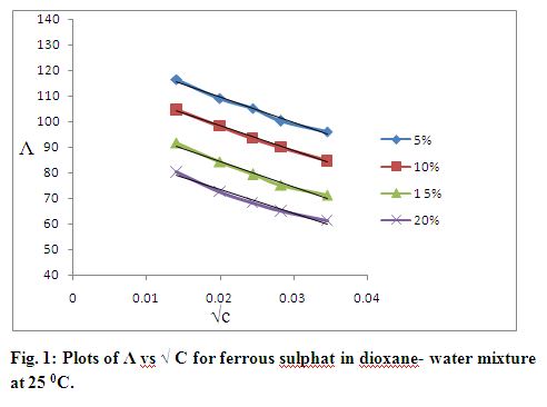
Where Λ0 is estimated from the Λ vs. c1/2 plot in Fig. 1 is 128.8. The Onsager limiting slope ‘S’ obtained from of Λ vs. c1/2 plot is 899.50.
This trial value Λ0 is used to compute E, and Λʹ. These values are used to calculate y and x by using equation ( 3.4 ), ( 3.7 ) and ( 3.5 ).
Then the series of calculations are made for a set of Λ0values. For calculation of , Λ׳ and the following values are needed.
T = 298 0K, D = 74.38, η = 0.009664 poise,
S = 899.50 and E1, E2
E1 = Z6 = 26 = 39.82
E2 = Z5 = 25 = 672.43
And, E = E1 Λ0 – E2
Using the value Λ0 = 128.8, E = 4455.82
= 116.50 / [128.8 – 899.50 (2.00 10-4 1/2]
= 0.998271
Λ׳ = Λ + S (cγ)1/2 – Ecγ log (cγ)
= 132.50
and the difference between Λ׳ – Λ0 = 3.69
if Λ0 = 132.0 is used, then = 0.9704 and Λ׳ = 132.241168.
and Λ׳ – Λ0 = 0.24
To fix Λ0, the difference between ( Λ׳ – Λ0) become less than 0.01.
For this we put Λ0= 132.21. Then = 0.9686, Λ׳ = 132.219586 and ( Λ׳ – Λ0 ) = 0.009 which is less than 0.01
Thus Λ0= 132.21 is fixed.
Using this Λ0 = 132.21 , , Λ׳, y and x are calculated for each c and Λ.
Calculation of y
y =
=
= 49.48
Calculation of x
x = Λ
–log =
= 0.789
x = Λ = 91.90
Thus the value of y and x are calculated in this manner for each concentration and equivalent conductance.
Then the initial y vs. x plot is made according to the equation y = J – KA x and the slope and intercept give KA and J respectively.
In this case, the initial value of KA and J is 251 and 22979 respectively.
From the value of J the values of aJ are obtained as follows:
J = Ϭ1 Λ0 + Ϭ2
Where
Ϭ1 = (k2 a2 b2 /12 c) [h (b) + 0.9074 + ln ( )
= Z6 [h (b) + 0.9074 + ln ( )]
Ϭ2 = α β + (11 β Ka /12 c 1/2) – (ka b β / 8 c 1/2 ) [1.0170 + ln ( ) ]
= z5 + z3a
– z2 (1.0170 + ln )
For 5% (w / w) dioxane – water mixture at 298 0K.
Ϭ1 = (229394405.6 a + 7.608005233 1014 a2– 1.26120645 1021 a3
+ 34.58317374 lna + 654.8660589)
Ϭ2 = 1.420509192 1010 a – 584.059164 lna – 10667.570558.
If Λ0 = 132.21, then
J = 4.451010 a + 1.0058 1017 a2– 1.67 1023 a3 + 3988.18 lna +75912.27
In this equation, different trial values of ‘a’ is used. The values of ‘a’ which fits the J equation is the desired ‘aJ’ value.
J = 22979 is obtained from the slope of y vs. x plot.
When
a = 16.50 10-8 cm, J = 22958
a = 16.55 10-8 cm, J = 23002
a = 16.52 10-8 cm, J = 22975
a = 16.53 10-8 cm, J = 22979
Thus the initial value of ‘aJ’ desired as 16.53 10-8 cm or 16.53 Å.
Then for higher approximation, γi ( i= 2 , 3 . . . ) is calculated by the equation
γi = Λ/ ( Λ0 – S ( cγi-1 )1/2 + Ecγi-1 log cγi-1 + J cγi-1)
where, on the right hand side, the first approximation for γ from (3.7) and the values just obtained for Λ0 and J are used. The calculation is repeated using equation (3.9) until γ (in) = γ (out) i.e., γn-1 = γn. At second time, Λ0 is fixed in same way.
If Λ0 = 132.17 is used in the calculation of γ in the above equation, then the constant γ׳ = 0.9643 and Λʹ׳ = 132.176245 for Λ =116.50 and c = 2.0 10-4. Then (Λʹ׳–Λ0) = 0.006 i.e., less than 0.01. Thus final Λ0 = 132.17 is obtained.
Using Λ0 = 132.17, J = 22979, Λ= 116.50 and γ1 = 0.9686, we get from the above equation:
= 0.9643
= 0.9643 using
Here, = = γ (constant).
Using this constant γ׳ (0.9643), Λʹ׳ = 132.176245 and y = 32.38 is obtained. Similarly different values of ‘y’are obtained for different Λ and c.
For the calculation of x at second time the equation of the mean activity coefficient is used.
= –
= {1/2 (2.0 10-4 22 + 2.0 10-4 22 )}
= 0.02966439
a = aJ (initial value) = 16.53 10-8 cm.
A = = = 0.552430962
B = = = 33778893.3
= –
= 0.8830799
= 0.7798
x = Λ = 0.7798 116.50
= 90.85
Thus different x values are calculated for different Λ and c. Thus final “y – x” plot is made. From this plot final KA and J are obtained.
The final aJ is obtained from final J. Using final Λ0 = 132.17 and
J = Ϭ1 Λ0 + Ϭ2
= 4.45 1010 a + 1.005 1017 a2 – 1.67 1023 a3+3986.8 lna + 75885.42
Final J = 24263
Different trial values of ‘a’ is used in this equation.
when
a = 17.55 10-8 cm, J = 23870
a = 17.95 10-8 cm, J = 24219
a = 17.98 10-8 cm, J = 24263
Thus, the final aJ = 17.98 Ǻ is obtained.
Now for FeSO4 in 5% (w/w) dioxane – water mixture the values are as follows:
Λ0 = 132.17, KA = 268, J = 24263 and aJ = 17.98 Å.
The initial y – x plot for 5% (w/ w) dioxane – water mixture at 298 0K is shown in Fig. 4.1. The final y – x plots for 5% (w/ w) dioxane – water mixture at 298 0K is shown in Fig. 4.2 and other plots are shown in Fig. 5 to 15.
The calculated values of γ, γ,׳ Λ’, Λ’׳, y , x , KA , J and aJ are shown in appendix Tables 10.1 to 12.16.
Calculation of aK from KA
ak are calculated from the slope of the plots of log KA vs. 1/ D according to the equation
KA = exp
From the log KA vs.1/ D (Fig.17) for FeSO4 in 5 % (w/ w) dioxane-water mixture at 298 0K .
Slope = = 113.00
Or, = = 113.00
Or, = 19.85 10-8 cm
= 19.85 A˚
CALCULATION OF THERMODYNAMIC PARAMETER
Calculation of ΔH0
From the plot of log KA vs. 1/ T (Fig.21) for FeSO4 in 5% ( w/w ) dioxane – water mixture.
Slope = = – 945.90
ΔH0 = – 8.316 2.303 (– 945.90) Joule mol-1
= 18115.64 Joule mol-1
= 18.12 k Joule mol-1
Calculation of ΔG0
From equation (1.51),
ΔG0 = – 2.303 RT log KA
Here, T = 2980K, log KA = 2.40
ΔG0 = – 8.316 2.303 298 2.40
= – 13697.33 Joule mol-1
= – 13.69 k J mol-1
Calculation of ΔS0
From equation (1.54), ΔS0 =
=
ΔS0298 = 106.75 J K-1 mol-1
Calculation of ΔGt0
ΔGt = ΔGt0( mixed solvent) – ΔGt0 ( water )
ΔG0 2980K for FeSO4 in water = – 13.05 kJ mol-1 42
ΔG0 2980K for CuSO4 in water = – 13.24 kJ mol-1 42
ΔG0 2980K for CdSO4 in water = – 13.43 kJ mol-1 42
ΔG02980K( 5% dioxane ) for FeSO4 = -13.69 kJ mol-1
ΔGt0 = –13.69 + 13.05 kJ mol-1
= – 0.64 kJ mol-1
= – 640 J mol-1
ΔG0t ( el ) = 4.184 166 ( – 0.0127) ( + )
For FeSO4 in 5 % dioxane-water mixture
ΔG0t ( el ) = 4.184 166 ( – 0.0127) ( + ) kJ mol-1
= 0.914 kJ mol-1
= 914 J mol-1
Where r1 = ionic radii of Fe2+ = 0.75 Ǻ and
r2 = ionic radii of SO42- = 2.30 Ǻ
ΔG0t ( ch ) = ΔGt0 – ΔG0t ( el )
= – 640 – 914 = – 1554 J mol-1
Calculation of Hydrodynamic Radii
The hydrodynamic radius for a cation and anion is given by
R+ =
R– =
To calculate and , the value of = 79.80 in water at 250C has been taken.43,44 The Λ0 values of FeSO4, CuSO4 and CdSO4 in water are 138.36, 135.43 and 141.65 respectively at 250C43,44 The anion transport number of infinite dilution was calculated by the equation.
t0– = and t0+ = (1 – t0–).
For FeSO4 in 5 wt. % dioxane- water mixture at 250C.
t0– = = = 0.58
and t0+ = ( 1- 0.58 ) = 0.42
Assuming t0+ to remain constant with solvent composition R+ and R– could be calculated at different solvent compositions.
= 0.42 132.17 = 55.51
= 132.17 – 55.51 = 76.66
R+ = = 3.06 Ǻ
R– = = 2.21 Ǻ
4. RESULTS AND DISCUSSION
The equivalent conductance (Λ) of ferrous sulphate, copper sulphate and cadmium sulphate solutions at different temperatures varying solvent compositions are listed in Table 2.1 to 2.12. Plots of Λ vs. √ C are shown in Fig. 1 to 3. The limiting Onsagar slope (S) was found from the slope of the resulting straight lines. Extrapolation of Λ at √C = 0 gave values of limiting equivalent conductance (Λ0) which were used in the Fuoss-Onsagar equation as a preliminary data.
4.1 ION-ASSOCIATION CONSTANTS
The ion – association constant (KA), for the following reaction
M2+ + SO42- ↔ M2+. SO42- (M = Fe, Cu, Cd)
were calculated from conductivity data according to the Fuoss-Onsagar conductance equation.40,41 The revised Fuoss-Onsgar equation for the equivalent conductance of the associated homologues electrolyte is given by
Λ = Λ0 – S(cγ) 1/2 + Ecγ log(cγ) + Jcγ – KA (cγ) f±2 Λ
where KA = (1 – γ) / c γ2
The values of Λ0, KA, J and aJ at different temperatures and solvent composition are summarized in table 3.1 to 3.3. Fig. 16 shows that the values of Λ0 decreased with decrease dielectric constant (D) of the medium. The ion-association constants (KA) values were found to increase with increase of organic portion of the solvent mixture. The KA values of CuSO4 found to at each temperature and at each solvent composition are larger than those of FeSO4 and the KA values of FeSO4 larger than those of CdSO4. The trend of the all KA values are shown below
SUMMERY
The conductance of three homologous electrolytes namely FeSO4, CuSO4 and CdSO4 is measured in dioxane-water mixtures at varying composition at different temperatures. The ion-association constant (KA) of the three electrolytes are found to increase with increase of organic portion in the solvent mixture and follow order at certain temperature.
CuSO4 > FeSO4 > CdSO4
The values of KA are found to increase with decreasing cation size. This result suggests that ion-association is cation size dependant. The KA values also increase with increase of temperature.
The changes of standard Gibbs free energy of ion – association are negative which shows that the association occurs thermodynamically spontaneously. The changes of standard entropies of ion – association are positive and decrease with increase of temperature. This phenomenon can be explained as the result of reduction of electric field of the associating ion. The positive values of standard enthalpy change reveals that the association is an endothermic process.
The change of standard Gibbs free energy of transfer (ΔGt0) from water to mixed solvent are always negative which suggests that the ion pair are in a lower energy-state in aqua-organic solvents than in water.The ΔG0t (ch) values for all the three electrolytes are formed negative which indicates spontaneous solvation and specific ion–solvent interaction. The values of ΔG0t ( el ) are positive for all the three electrolytes and magnitude decreases with increase of dielectric constant of the solvent mixture. The lower the values of ΔG0t ( el ) the greater is the electrostatic interaction between ion and total charges on the solvent molecules.
The walden products of all electrolytes in different solvent mixture are not constant which indicates that the stoke’s model of continuous solvent structure is not valid for the system. The walden products (Λ0η) for the three electrolytes follow the order
CdSO4 > FeSO4 > CuSO4
The walden products of CuSO4 only show positive temperature coefficient almost every solvent composition except 10% of dioxane-water mixture. This result shows that CuSO4 has the greatest structure making character than FeSO4 and CdSO4.
The values of aK are closer to the distance of closest approach, aJ and the values of aK as well as aJ for all the three electrolytes much larger than the sum of their lattice radii which indicates that the solvent molecules enter into the structure of the ion – pairs giving rise to solvation and formation of solvent separated ion pairs. The enhanced electric effect due to the double charges on each ion and the small size of Cu2+ gives rise to considerable polarization to a number .
ABSTRACT
Ion-association constant (KA), distance of closest approach (aJ) and thermodynamic parameters for several electrolytes namely ferrous sulphate, copper sulphate and cadmium sulphate were calculated from their conductance data in dioxane- water mixtures of varying compositions at temperature of 250C, 300C, 350C and 400C. The values of ion-association constants are increased with increase of dioxane content and it also increased with increase of temperature. The standard Gibbs free energy, entropy and enthalpy for the reaction M2+ + SO42- = M2+ SO42- were calculated from the temperature dependence of the ion-association constant. The standard free energy of transfer (G0t) from water to dioxane–water mixtures was calculated. The electrostatic and non-electrostatic contributions to the transfer free energy change, the free energy of transfer of individual ions in different solvent mixtures have been calculated. The solvated ionic radii have also been calculated. The distance closest of approach (aJ) of each solvated ion has been calculated. The walden products of the electrolytes in different solvent compositions were evaluated